Vladislav G. Polnikov, Fedor A. Pogarskii
A.M. Obukhov Institute of Atmospheric Physics of Russian Academy of Sciences, Moscow, 119017, Russia
Correspondence to: Vladislav G. Polnikov, A.M. Obukhov Institute of Atmospheric Physics of Russian Academy of Sciences, Moscow, 119017, Russia.
| Email: |  |
Copyright © 2012 Scientific & Academic Publishing. All Rights Reserved.
Abstract
Statistical processing was executed for measurements data from 14 buoys located in the Arabian Sea and the Bay of Bengal and for simulated data for wind and waves, adapted to the buoy points. For both kinds of data, histograms, probability functions, and frequency spectra were constructed and compared. The histograms show significant variation in space and dependence on the kind of their origin. That provides a corresponding impact on their regime characteristics for wind and wave fields in the area considered. Unlike histograms, spectral characteristics have more spatial uniformity. For both wind and wave fields, the main time-scale of variability is 1 year. Besides, both fields have evident variability scales of 40, 1, 1/2 and 1/3 days. Comparison of the spectra for measured and simulated series shows the informative preference of the latter, due to a noise of measurements.
Keywords:
Wind, Wave, Histogram, Probability Function, Spectra, Variability time-scales
Cite this paper: Vladislav G. Polnikov, Fedor A. Pogarskii, Short-Term Variability of Wind and Waves, Based on Buoy Measurements and Numerical Simulations in the Hindustan Area, Marine Science, Vol. 3 No. 2, 2013, pp. 48-53. doi: 10.5923/j.ms.20130302.02.
1. Introduction
The interest of studying variability of wind and wave fields is stipulated in scientific terms by the goals of understanding mechanisms of mechanical interaction between the atmosphere and ocean[1,2]. In applied terms, such studies are important for solving safety of navigation, coastal and marine industries, as well as the sustainable development of the resort activities and maintenance of ecological safety. To solve these problems, various numerical models are widely involved to the studies. Some of them provide restoration long-term wind fields (reanalysis)[3, 4] over the area; some others allow calculatingproper wind-wave fields[1, 2]. The fields obtained with simulations are the subject for comparison with the fields of observations, for example, on the basis of their statistical analysis. That allows assessing a quality of modelling, as well as a degree of variability of the fields studied, including their long-term trends[5, 6]. Relevance and accuracy limits of available numerical models are estimated by bringing systematic measurements of wind and wave fields. Among these there are the data of buoy stations, ships[7], and satellite measurements[8]. In this paper, we have used the data of buoy stations in the seas around Hindustan: the Arabian Sea and the Bay of Bengal (as a part of the Indian Ocean). This choice is due to amore general problem of research for long-term variabilityof wind and wave fields in the Indian Ocean as a whole[6].In particular, it is interesting to find out the scales of variability of wind and waves, basing on buoy data, and to construct the corresponding probability distribution functions. Then they are to be compared with those for the simulated wind and wave fields. Such a comparison allows us to evaluate an authenticity of the modelling fields, on the results of analysis of which, all further conclusions are built about wind and wave fields variability in the whole Indian Ocean[6]. In addition, these estimates are important for their use in practice of regional challenges noted above.
2. Data and Research Methodology
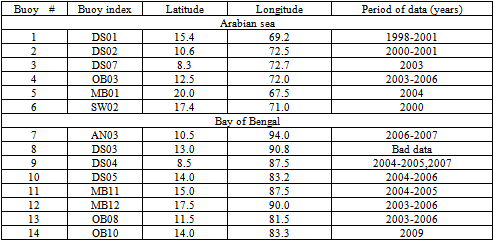
The measured data are three-hour time-series obtained at the buoy stations located in the Arabian Sea and the Bay of Bengal, Indian Ocean1. Given the need for comparison of these data with the results of numerical simulations, we have selected 14 stations located at a distance of over 150 kilometres of coastline, to avoid the impact of borders to modelling series. List of coordinates of these buoys and periods of more or less continuous measurements on them are given in the Tab. 1.For constructing histograms and probability functions, the real raw data are acceptable. However, to construct the frequency-spectra of the time-series for wind and waves, it was necessary to fill the gaps in these series to provide for a strict 3-hour equidistance of the measurements. For this purpose, for the gap points of wind series, the reanalysis ERA-Interim[9] was used. In the case of wave series, the results of numerical simulations of wind-wave field were used, calculated with the European wind-wave model WAM-cycle4[10].2 All the statistical characteristics were built for both field and simulated data. Then, the proper statistical characteristics for wind and wave fields were compared that determine the accuracy and relevance of the simulation results.Table 1. Information on the selected buoys measurements
 |
| |
|
3. Main Results
3.1. Wind Statistics
Normalized histograms for wind H(W) (in fact, the probability density function), obtained from measurements at 3 buoy stations, are shown in Figs. 1a,b.3The typical features of these histograms are as follows: (a) more irregularity of histogram in the Arabian sea, and (b) rather small probability for the winds more than 15 m/s. The corresponding probability functions F(W), obtained from the histograms H(W) by the formula[11] | (1) |
are shown in Figs. 2a,b. Recall that in the case when probability function F(W) is obtained on the basis of a sufficiently large (i.e. statistically relevant) sample, the value of F(W0) is the probability for the random variable W to exceed the fixed value W0 in a statistical ensemble for W. Extrapolation of F(W) to the fixed higher value W = Wm allows to estimate the return time for value Wm[11].An obvious difference between the shown probability functions F(W) is a higher probability of strong winds in the Arabian Sea. It must be assumed that the strong winds are associated with the monsoon, the strength of which in the Arabian Sea was higher than in the Bay of Bengal (during the observation period).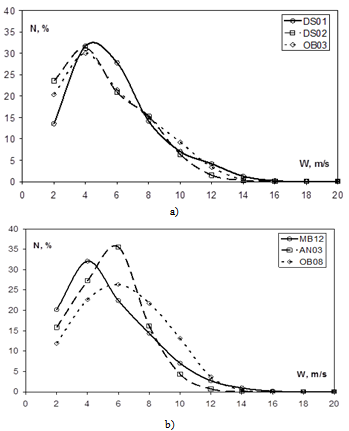 | Figure 1. The wind histograms for 3 buoys: a) in the Arabian sea; b) in the Bay of Bengal |
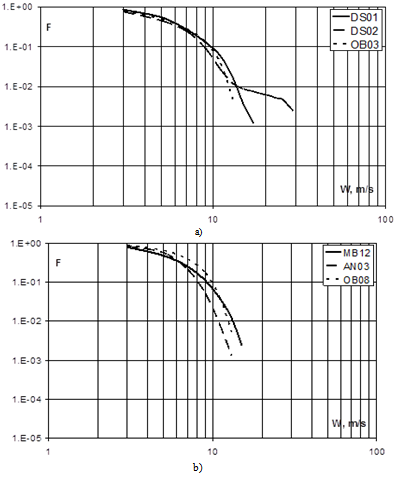 | Figure 2. The probability function F(W) of the wind for 3 buoys:a) in the Arabian sea; b) in the Bay of Bengal |
The results obtained are interesting to compare with the distribution functions for the reanalysis wind data adapted to the proper buoys points (Figs. 3 a,b). In these figures, it is notable a significant reduction in the probability of wind values more than 15 m/s in the reanalysis data, compared with the measured data (especially the Arabian Sea). The reason for this difference lies precisely in the fact that, according to the construction technique, the reanalysis wind field is smoother and virtually is devoid of a momentary increase of the wind, caused by cyclones. 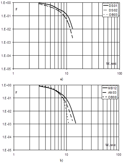 | Figure 3. The probability function F(W) of the wind reanalysisat points of 3 buoys: a) in the Arabian sea; b) in the Bay of Bengal |
Furthermore, if one tries to assess the return value of strong winds, basing of the constructed functions F(W), the probability function for the reanalysis gives lower return values. So, extrapolating F(W) in Fig. 2a, one finds the occurrence of extreme wind one time in 50 years (when F(W) ≈ 10-5) of the order of 35-40 m/s in the Arabian Sea. The same value obtained from Fig. 3a gives the return wind of about 20 m/s. For the case of the Bay of Bengal (as shown in Figs. 2b and 3b), one can get 25-30 m/s and 20 m/s, respectively.From the said it follows important practical conclusion: to obtain a reliable statistics of wind, the direct measurements are preferred compared to the results of a numerical simulation.
3.2. Statistics of Waves
Similar results for the significant wave height HS of wind-waves are shown in Figs. 4a,b (due to limited space, the distribution functions are given only). Comparison Figs. 4a,b with Figs. 2a,b indicate that the wave statistics is defined not only by the statistics of wind but by the area geometry as well. The latter means that the fetch of the wind plays the role in the statistics of waves, whilst statistics of the wind could be the same.Indeed, despite the fact that the probability of wind value of 15 m/s on buoys DS01 and MB12 are comparable, high waves (HS> 6m) in the Arabian Sea are more probable than in the Bay of Bengal at the appropriate points. Clearly, in the latter case, the limited area of the bay, compared to one of the open sea, plays the role.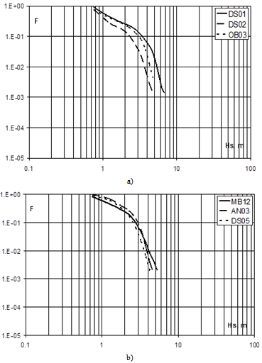 | Figure 4. The probability function F(HS) of the measured wind-waveheights: a) in the Arabian sea; b) in the Bay of Bengal |
As to the return value of extreme waves 1 time in 50 years, according to Figs. 4a,b, the significant wave height can reach values HS = 12-15m in the Arabian Sea, while in the Bay of Bengal it does 8-10m, only. In conclusion for wave statistics, say about the distribution function of wave heights, which follows from the results of simulations, shown in Figs. 5a,b.From these figures it is seen a good agreement between probability functions for both the empirical and simulated wave heights. It is apparently caused by a considerable inertia of waves compared to the variability of wind. In practical terms, this suggests a possibility of using the simulated data to estimate the statistical characteristics of the wave field.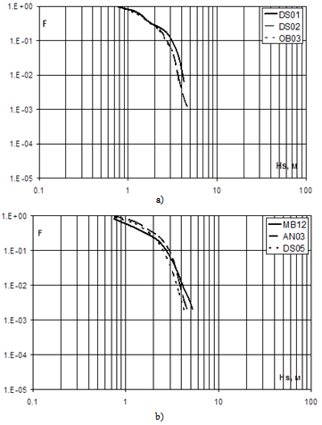 | Figure 5. The probability function F(HS) of the simulated wind-wave heights:a) in the Arabian sea; b)in the Bay of Bengal |
3.3. Spectra of the Wind Speed Series
The frequency spectra of random time-series provide information on distribution of the variation-intensity along the time scales. Moreover, the spectral shapes are of reasonable physical interest, as far as it is the spectral characteristics that can be obtained theoretically from the equations of motion. Thus, a study of the spectra provides a basis for a testing theoretical constructs and stimulating new constructions. In our case, the spectra were calculated by using the Yule-Walker auto-regression method (software Sptool in the shell of the MATLAB(c)) applied to the 3-hour series of both buoy measurements data and model calculations. In our case, the confidence intervals in logarithmic coordinates are about ± 30%.Typical results for the buoy data are shown in Figs. 6 a, b.The common features of these two types of spectra (typical of all the buoys mentioned above), hereinafter referred to as the empirical and model ones, are as follows:1) well highlighted scale of 1 year;2) noticeable scale of 40 days;3) slight changing spectrum intensity in the range of 50 to 10 days;4) power spectrum shape of the form  | (2) |
for the periods less than 10 days;5) presence of sharp peaks at scales of 1, 1/2, and 1/3 days.Differences between the empirical and model spectra are as follows.First, for the periods less than 1 day, a very noticeable noise presents in the empirical spectra (it is almost the white noise with an equal intensity of spectrum through the frequency scale). The proper noise is completely absent in the model spectra.Second, the slope-index n of the spectrum, given by formula (2), is equal to 1.4-1.5 for the empirical spectra in the range of periods of 10 to 2 days, only. The same index is equal to 1.5-1.6 for the model spectra in the wider range of 10 to 0.3 days.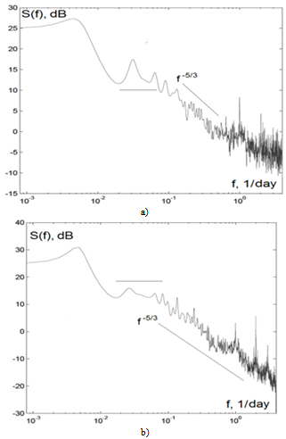 | Figure 6. The wind-speed spectra: a) measurements at buoy DS01; a) wind reanalysis for the point of buoy DS01. Strait lines are simbolizing the inclination of different parts of the spectra |
The obvious reason for the noise of the empirical data is a natural oscillation of the measuring buoy-platform. Due to this, distortions occur in the slope of spectrum, determined by index n. It is however important to note that in the both cases, exponent n is very close to the theoretical index of the isotropic Obukhov-kind turbulence, for which it should be n = 5/3 = 1.66[11]. This fact is quite plausible, and that allows us to trust the results obtained.Besides, from a practical point of view, it is essential to note that the model spectra are closer to the theoretical ones, due to they are less noisy. This fact indicates that the model results are preferable to getting reliable estimates of the spectral characteristics studied.In our case, we do not consider the ordinary frequency spectra of instantaneous wave heights, fairly well studied by numerous authors[1, 2]. Here we do study the spectra of statistical characteristic of the wave height: the spectra of significant wave height HS determined from the ordinary wave spectra by formula
 | (3) |
whilst the spectra  at each space point (i, j) and time moment (t) are calculated with the wind-wave model WAM(cycle4). Such a kind studies are not numerous (see references in[6]), and each of them is of considerable interest.
 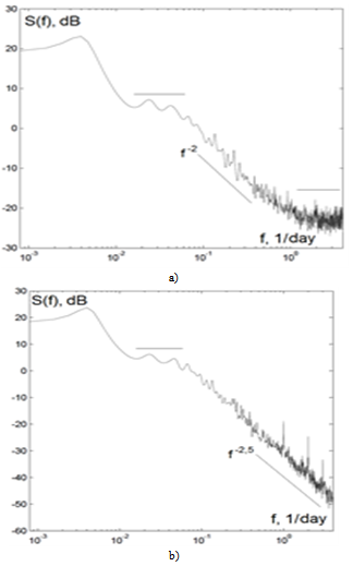 | Figure 7. The significant wave-heightspectra: a) measurements at buoy DS01; b) wave simulations for the point of buoy DS01. For legend see Fig. 6 |
Typical spectra of the series of HS, obtained from buoy and model data are shown in Figs. 7 a, b. As one can see from Figs. 7, common features of the empirical and model spectra for HS are as follows:1) well highlighted scale of 1 year;2) very weak variation of the spectrum intensity on the scales 50 to 10 days;3) power spectrum shape of form (2), starting for periods less than 10 days; Differences between the empirical and model spectra are as follows:1) for the range of the periods less of 2-3 days, a remarkable noise presents in the empirical spectra, transforming to the white noise spectrum on the scale less than 1 day. This noise is virtually absent in the model spectra due to no physical reason for it in a numerical model;2) the slope-index of the spectrum n, determined by formula (2), is equal to 2.0-2.2 for the empirical spectra in the range of periods 10 to 3 days. The same index is equal to 2.5-2.6.3 for the model spectra in the range 10 to 0.3 days;3) In the model spectra there are clearly marked peaks at scales 1, 1/2, and 1/3 days. These peaks are buried in the noise for the empirical spectra. As in the case of spectra for wind speed, the cause of all these differences for the spectrum of wave height is the measurement noise. Therefore, we can state that the model series of significant wave heights are preferred to perform their spectral analysis, with respect to buoy data.On the background of the apparent scale of variability of one year, there are not obvious reasons of appearing the "shelf" in the spectrum for wave heights, taking place in the range 50 to 10 days. There is not obvious, as well, the nature of setting the power-law decay spectra for significant wave height HS in the range of periods less than 10 days. In this study, we only raise these questions, and their solution lies in the frame of constructing the corresponding theoretical models.
4. Conclusions
The set of new results is the following.1. Direct measurements are preferred with respect to simulated data for constructing histograms and probability functions, including their statistical moments, for both the wind and wave height fields. All probability functions for simulated data underestimate the probability of extreme values of the variables studied.2. The statistical characteristics mentioned above have significant spatial variability, especially for the wind values, which requires an independent and separate study of them for each geographical area.In particular, it was found that the extreme wind appearing once for 50 years is of the order of 40 m/s in the Arabian Sea. In the Bay of Bengal, this amount is about 30 m/s.Extreme wave height HS appearing once for 50 years is of the order of 15m in the Arabian Sea and of 10m in the Bay of Bengal.3. Spectral characteristics of the empirical and model series of wind and waves are less variable in space. In necessity of constructing regionalized spectra, this fact allows the averaging of the original series on large spatial scales limited by the properly ranged geographical areas.4. The spectra of empirical series (buoy data) are heavily distorted by the measurement noise which is significant on the scale of periods less than 1 day. Therefore, for the purpose of spectral analysis, the modelling series of wind and wave heights are more preferable than buoy data.5. In the Arabian Sea and the Bay of Bengal, the highlighted scales of variability for wind are as follows: 1 year, 40 days, 1 day, 1/2 and 1/3 days. For the significant wave height, the highlighted scales are: 1 year, 1 day, 1/2 and 1/3 days.6. The spectrum of the simulated data for wind (reanalysis) has the decaying power-law with exponent n ≈ 5/3 for the periods less than 10 days, and the spectrum of the simulated significant wave height has n ≈ 5/2 in the same period domain. These results are more reliable just for the simulated data than for measured ones.7. In the spectrum of significant wave height, the spectral shape has a weak dependence on frequency (the white-noise spectral shape) in the domain 50 to 10 days, the nature of which is still unknown. A similar, but less pronounced feature takes place in the spectrum for wind speed.
ACKNOWLEDGEMENTS
We thank our Indian colleagues:Dr. P. Vethamony, Mrs. S. Samiksha, and Mrs. R.Rashmi from the Indian Institute of Oceanography (Goa, India) for a kind providing the buoy data. We are grateful to our chief, academician G.S. Golitsyn for his recommendation to execute this study. The work was supported by the State Contract # 11.519.11.5023 with the Ministry of Education and Science of the Russian Federation.
Notes
1. These data were kindly provided by our Indian colleagues of the project.2. This choice of the wind reanalysis and wave model was provided by the task of the general project(see acknowledgement).3. Hereafter we show results for 3 buoys in each region, only. It is due to similarity of statistics and need of clearance of the plots.
References
| [1] | Efimov, V. V., and V. G. Polnikov, Numerical simulation of wind waves (in Russian), “Naukovadumka” publishing house, Kiev, 1991. |
| [2] | Komen, G. L., L. Cavaleri, M. Donelan et al., Dynamics and Modelling of Ocean Waves, Cambridge University Press, UK, 1994. |
| [3] | Rubinstein, K. G., and A.M. Sterin, “Comparison of the results of reanalysis with aerological data” (in Russian), Izvestiya, Atmospheric and Oceanic Physics, v.. 38, pp. 301-315, 2004. |
| [4] | Saha, S., et al., “The NCEP climate forecast system reanalysis”, Bull. Am. Meteor. Soc., v. 91. pp. 1015-1057, 2010. |
| [5] | Sterl, A., G. J. Komen, and P. D. Cotton, “15 years global wave hindcast using ERA winds”, Journal of Geophysical Research, v.. 103, pp. 5477-5492, 1998. |
| [6] | Pogarsky, F.A., V.G. Polnikov, and S.A. Sannasiraj, “Joint analysis of the wind and wave-field variability in the Indian Ocean area for 1998–2009” (Eng. Transl.), Izvestiya, Atmospheric and Oceanic Physics, v. 48,pp. 639-656, 2012, DOI: 10.1134/S0001433812060114. |
| [7] | Gulev, S.K., V. Grigorieva, “Variability of the Winter Wind Waves and Swell in the North Atlantic and North Pacific as Revealed by the Voluntary Observing Ship Data”, J. Climate, v.19, pp. 5667-5685, 2006. |
| [8] | Young I.R., S. Zieger, A.V. Babanin, “Global Trends in Wind Speed and Wave Height”, Science, v. 332,pp. 451-455, 2011. |
| [9] | Site http://www.ecmwf.int/research/era/do/get/era-interim. |
| [10] | The WAMDI Group,“The WAM – a third generation ocean wave prediction model”,J. Phys. Oceanogr.,v.18, pp. 1775-1810, 1988. |
| [11] | Petrauskas C., P. Aagaard, “Extrapolation of historical storm data for estimating design-wave heights”, J. Soc. Petroleum Eng.,v. 11, N 1, 1971. |
| [12] | Monin, A. S., A.M. Yaglom, Statistical Fluid Mechanics: Mechanics of Turbulence, v. 1. The MIT Press, Cambridge, Massachusetts, and London, England, 1971. |
 Abstract
 Reference
 Full-Text PDF
 Full-text HTML