Soovoojeet Jana , T. K. Kar
Department of Mathematics, Bengal Engineering and Science University, Shibpur, Howrah, 711103, West Bengal, India
Correspondence to: Soovoojeet Jana , Department of Mathematics, Bengal Engineering and Science University, Shibpur, Howrah, 711103, West Bengal, India.
| Email: |  |
Copyright © 2012 Scientific & Academic Publishing. All Rights Reserved.
Abstract
This paper deals with the optimal allocation of an ocean space for the purposes of fishing and ecotourism management. Here we have considered that one portion of the region to be used for ecotourism and rest of the portion to be used for fishery management. Our main aim of the problem is to optimize the total profit earned from both fishery and ecotourism and for this purpose we have used optimal control technique. Some necessary and sufficient conditions are established for the existence of different equilibria, their stability and Hopf bifurcations of this optimal control problem. It is observed that the result depend strongly on different catch rate functions of the fishery.
Keywords:
Ecotourism, Harvesting, Adjustment Cost, Optimal Control, Stability
1. Introduction
The excessive and unsustainable exploitation of our marine resources has led to the promotion of marine reserves as a fishery management tool. Marine protected areas (MPAs) where fishing is restricted or prohibited, can offer for the recovery of exploited stock and fishery enhancement. The objectives pursued can generally be classified under one of the three following catagories: ecosystem preservation, the management of commercial fisheries and (or) development of recreational activities. But to the authors’ knowledge there is no such work on ecotourism management in the marine reserved portion. But we do think that it is quiet more beneficial to the society if we create ecotourism in the reserved portion of the ocean with the fishery management in the other portion.Conrad (1999) showed that, in the absence of ecological uncertainity and in the context of optimal harvesting, reserves generate no economic benefits to fishermen. Such result coincides with the perspective of many fishermen and also some economists. However Luke et al. (1998) asserted that MPAs can be viewed as a kind of insurance against scientific uncertainity, stock assessments or regulation errors. Kar and Matsuda (2008) consider a bioeconomic model of a single species fishery with a marine reserve. Their study examines the impact of the creation of the marine protested areas (MPAs), from both economic and biological perspectives. In particular, they examined the effects of protected patches and harvesting on resource populations. They conclude that the protected patches are an effective means of conserving resource populations, even though extinction can not be prevented in all cases. Hartmann et al. (2007) investigatede the economic optimality of implementing an MPA to get more informative data about fish population, thereby arrising a better management strategy. Powell et al. (2002), examined the contribution of fully protected tropical marine reserves to fishery enhancement by modelling marine reserves fishery linkages. The consequences of reserve establishment on the long run equilibrium fish biomass and fishery catch levels are evaluated. They also concluded that marine reserves are an important component of sustainable tropical fisheries management and reserves will be most effective when coupled with fishing effort controls in adjacent fisheries.[1] In their books Clark (1990) and Kot (2001) present mathematical study of population ecology with harvesting. Recently Kar and Chakraborty (2009) describes marine reserves and its consequences as a fisheries management tool. But to the authours knowledge no attempt has been made to consider the ecotourism management in the reserved portion of the fishery. [2]In our present work we divide the total region i.e. total available ocean spaces into two regions: one is the fishing zone and the other one is no fishing zone. The no fishing zone should be used for the ecotourism purpose by arranging boating, some water sports etc. Also it is possible to make the region for ecotourism purpose in another way. In a comparative higher region of a sea or big lake can be made man-made island where eco-tourism should be taken place by means of tourism, gardening, aquarium etc. It is very useful that the investment cost for the creation of ecotourism is quiet high though thereafter the cost will be less than that of the fishery.  | Figure 1. Conseptual diagram of an ocean region allocated for harvesting zone and ecotourism zone |
For modelling purpose let us assume that  be the total ocean area where both fishing and eco-tourism are done and
  be the portion where only ecotourism takes place. Thus obviously the total region for eco-tourism would be proportional to
  and hence it is taken as
  with
with  is a positive parameter. Also let
  be the intrinsic growth rate of the population species in the fishery system and
  be their catching rate. Obviously the carrying capacity for this population would be
  Hence our mathematical model of the single species population is:
 | (1.1) |
Let  be the total amount of investment applied for eco-tourism purpose. Now if
  be the proportion parameter i.e. if the portion
  of the total investment cost used for preparing the non fishing zone for eco-tourism zone. The next amount of investment i.e.
  is applied to make some kind of publicity among the tourists so that they are attracted to visit that place. Now we reconstruct our mathematical model as follows:
 | (1.2) |
with the conditions  Obviously the secondary cost i.e.
  will be proportional to the income due to the eco-tourism. Moreover the income due to the eco-tourism will be prportional to the area where eco-tourism is done. Thus we may take the total income due to the eco-tourism as
  Next we calculate the total amount of profit due to the fishery system. Let us assume that
  be the harvesting effort,
  be the cost for each unit of harvesting and
  be the selling price of each unit of fish due to the harvesting. Thus total economic rent or profit due to the fishery management is:
  In figure 1, we present a conceptual diagram of the considered system.Moreover there is a cost which is known as "adjustment cost" (see Stollery (1986), Feichtinger and Sorger (1986), Vilchez et al (2004) etc.) is taken as the quadratic function of the variable
  This adjustment cost can be interpreted as the cost initiating with the cost due to the eco-tourism. This cost is taken as quadratic function of the variable
  since over investment for the eco-tourism may be the cause for the loss in both eco-tourism and harvesting. Now we form the optimal control problem with the following Jacobian
 | (1.3) |
subject to the differential equations (1.2).Here  is the discount rate associated with the infinite horizon optimal control problem. Clearly (1.3) is an optimal control problem with two state variables namely
  and
and  and one control variable namely
  We use Pontryagain's maximum principle to solve the above optimal control problem. At first we form
  the current value Hamiltonian of our problem as follows:
  | (1.4) |
where  and
and  are co-state variables.Now from the optimality condition we have,
  which gives,
  i.e.
i.e.  | (1.5) |
Also we get the transversality conditions of the system as follows:  Now together with the state equations and the transversality equations we can write our system as a combination of four first order differential equations from which we can get the required solution of our system. Now these equations are as follows:
 | (1.6) |
Our paper is organized in the following way. The sections 2, 3 and 4 deal with the analysis of the system for three different harvesting functions namely, Schaefer catching function, Cobb-Douglous catching function and Michaelis–Menten type of harvesting respectively. In section 5, we give some numerical simulations and in the last section we draw some conclusions from our throughout analysis.
2. Analysis for 
Schaefer (1957) introduce the harvesting form as catch-per-unit effort. For this here we take harvesting in the form  where
where  is the catchibility coefficient. Using the optimality condition, we have from (1.6) the reduced four first order differential equations as follows:
 | (2.1) |
Now we try to find the non-negative equilibria of the system of differential equations (2.1). Clearly we see that there may be two equilibria of the system (2.1). One is  and other is
  where
where  is given by as follows:
 | (2.2) |
For both economical and biological context the necessary and sufficient condition for the existance of the above equilibrium is given by  If
If  then the density of the population
  will be negative and so there will be no population in the system. This case may be occured due to the over harvesing than the population intrinsic growth rate and in this case the system will be collapsed. So to remain the system alive we must take the harvesting effort,
  less than
2.1. Stability Analysis of the System.
In this subsection we now describe the local stability and bifurcation of our system around two equilibria  and
and  in the following theorems.Theorem 1. The system (2.1) is unstable around the equilibrium
  Proof. The characteristic equation to the system (2.1) at its equilibrium
  is given by:
 i.e. the eigenvalues are given by:
  and
and  Since the real part of
  are positive hence we may conclude that the system (2.1) is unstable at the equilibrium
 Next we shall study the local stability criterion of the system (2.1) at the equilibrium
  For this we now try to find the characteristic roots of (2.1) at
  After some simple manipulation we get the characteristic equation of (2.1) at
  as
as  where
where 


 Now let us calculate the value of
  We have,
  where
where  and
and  Thus for
  where
where  is the positive value of
  of the equation
  we have,
  Now we are in a position to state the following two theorems related to the local stability and Hopf bifurcation to the system (2.1) which can be easily proved by using Routh-Hurwitz criterion.Theorem 2. The system (2.1) is locally asymptotically stable at
  if
if  and
and  hold provided
  .Theorem 3. The system (2.1) undergoes through a Hopf bifurcation at the equilibrium
  for
for  .
.
2.2. Influence of Some Important Parameters to the Equilibrium 
We now intend to see the influence of some important parameters namely  and
and  at the equilibrium level of the system (2.1).We see that
  and
and  Thus at the equilibrium
  the value of
  decreases(increases) as the parameter
  increases(decreases) where as the value of
  increases(decreases) as
  increases(decreases) although
  has no effect on the shadow price
  Also,
Also, and
and  It is obvious that
  for
for  and
and  for
for  provided
  where
where  Thus it is concluded that at
 decreases(increases) and
  increases(decreases) as
  increases(decreases) where as in
 increases(decreases) and for

 decreases(increases) as
  increases(decreases).Next,
 Thus we conclude, at
 and
and  both increases(decreases) where as the shadow price
  decreases(increases) as the intrinsic growth rate
  increases(decreases).Ultimately,
  and
and  Thus at
  both
both  and
and  decreases(increases) as the parameter
  increases(decreases) although
  has no influence on the population density

3. Analysis of the System for Cobb-Douglous Catching Function 
Again using the optimality condition  we get the reduced form of system of differential equations (1.6) as follows:
 | (3.1) |
Next we try to find all possible non-negative equilibria of the above system by making the right hand side of above equation (3.1) equals to zero. Clearly the system (3.1) has three different equilibria and among them the first two are respectively  and
and  where
where  and
and  are the roots of the equation
  The rest equilibrium is given by
  where
where 

 Now both equilibria
  and
and  are either feasible or imaginary depending on the nature of
  If
If  then both equilibria
  and
and  are feasible otherwise they are imaginary. Now both the equilibria
  and
and  has only biological impact since the population are able to survive. On the otherhand these equilibria have no economic meaning due to the aqualture and only economic profit may be gained by the harvesting.
3.1. Stability Analysis
In this section we shall discuss the stability of the system (3.1) at different equilibria. In the following theorem we study the local stability of the system around  and
and  Next we study the same around
  Theorem 4. The system (3.1) is unstable around both the equilibria
  and
and  Proof. The characteristic equation to the system (3.1) at the equilibrium
  is given by:
 | (3.2) |
where, 


 Since here
  is negative then using Routh-Hurwitz criterion for stability we may say that at least one eigenvalue of the system (3.1) at the equilibrium
  is positive. Hence the system is unstable around
  Similarly replacing
  by
by  in the characteristing equation (3.2) we can obtain the characteristic equation of (3.1) around
  The coefficient of third degree term of that characteristic equation also will be
  Thus with the help of previous argument we can conclude that the equilibrium
  is also unstable. Hence the theorem.In the next theorem we will study the stability of the other equilibrium
  of the system (3.1)Theorem 5. The system (3.1) is unstable around the equilibrium
  Proof. The characteristic equation of the system (3.1) at the equilibrium
  can be written as follows:
 | (3.3) |
where 


 The characteristic equation (3.3) shows us that at least one eigen value of this characteristic equation is positive (using Routh Hurwitz critiaria for a polynomial equation of degree four). Hence the system (3.1) is unstable around its equilibrium
  Hence the theorem. Note. It is evident that if the catching would be of the form of Cobb-Douglous production function then always ststem would be unstable around its all possible feasible equilibria.
4. Analysis for 
Here we take the catching function of Michaelis–Menten type i.e. of the form  where
where  is the catchibility coefficient and
  are the Michaelis–Menten constants. So from (1.6) we have the four first order differential equations which can be deduced for harvesting by Michaelis–Menten type by using the optimal conditions are as follows:
 | (4.1) |
Next we try to find the possible non-negative equilibria of the system (4.1) by making right hand side of system (4.1) equal to zero. We are interested about the interior equilibrium of the system (4.1) although we always have  at the equilibrium. So let us denote the non zero value of
  at the interior equilibrium of the system (4.1). Let
  where
where  is the positive root of the equation
  | (4.2) |
where,


 and
and Clearly a sufficient condition that (4.2) has only one positive root is
  and
and  hold simultaneously. Also
  and
and  Thus the equilibrium
  is always nonnegative if (4.2) has one positive root and
4.1. Stability Analysis
Here we now discuss the criteria for local stability and examine if there will be any bifurcation at the equilibrium  of the system (4.1). The characteristic equation to the system (4.1) around its equilibrium
  is given by:
  | (4.3) |
where 


 and
and  Next we use the well known Routh-Hurwitz criteria to find the nature of the stability of the system around its equilibrium
  For this at first we define the following quantities:

 Now we state the following theorem in connection with the local stability criteria to the system (4.1) around its equilibrium point
  which can be proved by using the well known Routh-Hurwitz criterion for the local stability.Theorem 6. If all of
  and
and  are positive then the system (4.1) is locally asymptotically stable around
  where as if at least one of them is negative then the system (4.1) is unstable around
  .
.
5. Numerical Simulation
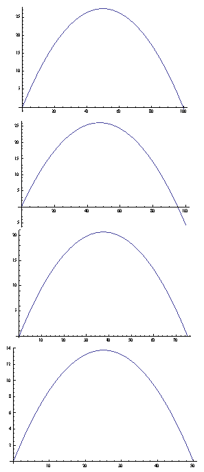 | Figure 2. Graph of the population biomass for  respectively where respectively where  is taken along the horizontal axis and the increment of is taken along the horizontal axis and the increment of  is taken along the verticle axis is taken along the verticle axis |
In this section we not only verify our analytical results through computer simulation but also we present some realistic phenomena for different parameter values.First we check the population biomass level for different value of the parameter  which is associated with the eco-tourism region
  . For the simulation purpose we take
  and four different values of
  namely
  and 10 with fixed value of
  as 5 units. In figure 2, we present the phenomena and see that higher values of
  makes to decrease population biomass quickly.Next we draw the graph for population growth curve and different catching function for different effort. Here for simulation we take,
  Also we take a fixed value of
  In figure 3, 4 and 5 we represent these phenomena for different effort and different harvesting rate respectively.
 | Figure 3. Graph for catching according to Schaefer catching function where  is taken along the horizontal axis and is taken along the horizontal axis and  is taken along the verticle axis is taken along the verticle axis |
 | Figure 4. Graph for catching according to Cobb-Douglous catching function where  is taken along the horizontal axis and is taken along the horizontal axis and  is taken along the verticle axis is taken along the verticle axis |
 | Figure 5. Graph for catching according to Michaelis–Menten catching function where  is taken along the horizontal axis and is taken along the horizontal axis and  is taken along the verticle axis is taken along the verticle axis |
The above three figures indicate the biomass of the population at the equilibrium level when we use different rate of harvesting. It is seen that the worst population density would be for catching according to Cobb-Douglus production function. Again catching according to the Michaelis–Menten rule gives the best result because here we can control both population biomass and total harvesting populations together since there are two extra control parameter namely  in this type of harvesting.
6. Conclusions
For a fishery manager the management objective is to maximize the rent of the fishery using certain management tools. On the otherhand long term resource conservation is also very much essential for our future generation as well. Under this circumstences marine reserve (where fishing is strictly prohibited) may be considered as an essential tool for this management purposes. We can develop ecotourism to overcome dilemma between the need for long term resource conservation and the immidiate necessity to provide jobs and income to the local population. In the present work we consider one portion of the available region to be used for ecotourism purpose (where fishing is not permitted) and the rest part to be used for fishery management. Here the region which is considered for ecotourism purpose is not a constant region. In fact this region is proportional to a particular area  whose cost to make it suitable for tourism purpose is known. Also the investment cost to this zone is divided into two parts: one part is applied to make the zone usable for tourism and the rest part is used as secondary cost to make the zone more attractive. Obviously this secondary cost would be proportional to the profit earn from the tourism purpose. Our main aim is to maximize the total profit from both the fishery and ecotourism. This type of simultaneous fishery and ecotourism policy would be very helpful to marine areas particularly nearby of any coastal areas or bank of the see. The idea of simultaneous fishing and ecotourism help to maintain equaility in the marine population. Thus to describe marine ecology our analysis would be very handful.Here we consider three types of catch rate functions, the Schaefer catching function
  the Cobb-Douglous production function
  and the Michaelis–Menten type catching which is of the form
  We analyze the stability of the systems at all feasible optimal equilibria. Among all the catching function the Michaelis–Menten type catching i.e.
  is most suitable catching function because in this case neither population nor harvesting effort go to infinity. Again it is evident from our throughout analysis that at the optimum equilibrium level the cost for the eco-tourism is zero.When we harvest according to the Schaefer catching function
  the system (2.1) gives two optimal equilibria, one is the population free equilibrium
  and another is
  If the growth rate of the population is less than the harvesting, then the system goes to a population free position and in this case system goes to the equilibrium
  which is a saddle point. Along
  all the trajectories except the trajectory along
  axis repel from
  The trajectory along
  axis attracted at
  due to the high harvesting rate as well as lower growth rate. Again the optimal equilibrium
  is conditionally locally asymptotically stable and for a critical value of
  the system (2.1) undergoes through a Hopf bifurcation. We see that when we use the Cobb-Douglous production function as the catching function then the reduced system has three possible non negative equilibria depending upon some parametric conditions and the system is unstable in nature around its all of those three possible equilibria. This is possibly due to the rate of the harvesting as the quadratic function of the fishing effort. Since harvesting is occurring at a rate of
  the population decreases always and this causes the increasing of the space for eco-tourism. Thus this type of harvesting never stabilize the population density and the eco-tourism region.Next when we use Michaelis–Menten type harvesting then the harvesting function is not only proportional to the harvesting effort and the stock of the population biomass but also it is inversely proportional to the joint effect of the harvesting effort and population biomass. In this type of Harvesting we also obtain more than one equilibria but we are interested to examine the system nature around the interior one and so we omit the others from our discussion. We find the local asymptotic stability criteria of the reduced optimal system around that interior equilibrium
  and see that it is conditionally stable there. Other functional form embodies like either
  or
or  has the following defects: (i) assumes random search for fish, (ii) assumes equal likelihood of being captured for every fish, (iii) there is unbounded linear increase in
  with respect to
  for a fixed
  (iv) there is unbounded linear increase in
  with respect to
  for a fixed
  etc. But those unrealistic features can be largely removed by adapting the alternative functional form of harvesting type of harvesting
  Hence this type of functional form is the best for both biological and economical context. In traditional way we use to harvest a population species to get some benefit from it. But over harvesting and unconsciousness harvesting causes the imbalance of natural resource of life because it may be the cause for the extinction of one or more species. Therefore to conserve the population for the future generation we may introduce some marine reserve where fishery may not be permitted but reserved region may be used for the purpose of the ecotourism. This ecotourism is economically profitable for the local people as wll as the government. In this way we see that eco-tourism is not only economically beneficial but also biologically strongly essential and this would make a balance of the population level in marine ecology.
ACKNOWLEDGEMENTS
Research of Soovoojeet Jana is financially supported by University Grants Commission, Government of India (F. 11-2/2002 (SA-1) dated 19 August, 2011). [3]
References
| [1] | J. M. Conrrad, The bioeconomics of marine sanctuaries, Journal of Bioeconomics, 1, 206-217, (1999). |
| [2] | T. Luke, C.W. Clark, M. Manget and G. R. Munro, Implementing the precautionary principles in fisheries management through marine reserves, Ecological Applications, 8(1), 1998, 72-78. |
| [3] | T. K. Kar and H. Matsuda, A bioeconomic model of a single species fishery with a marine reserve, Journal of Enviornmental Management, 86, 2008, 171-180. |
| [4] | K. Hartmann, L. Bode and P. Armsworth, The economic optimality of learning from marine protected areas, ANZIAM, 48, 2007, 307-329. |
| [5] | I. Rodwell and E. Barbier, A model of tropical marine reserve-fishing linkages, Natural Resource Modelling, 15(4), 2002 453-486. |
| [6] | T. K. Kar and K. Chakraborty, Marine reserves and its consequences as a fisheries management tool, World Journal of Modelling and Simulation, 5(2), 2009, 83-95. |
| [7] | M. L. Vilchez, F. Velasco and I. Herrero, An optimal control problem with Hopf bifurcations: an application to the striped venus fishery in the Gulf of Cadiz, Fisheries Research, 67, 2004, 295-306. |
| [8] | K. R. Stollery, Monopsony processing in an open access fishery, Marine Resource Economics, 3(4), 1986, 331-351. |
| [9] | G. Feichtinger and G. Sorger, Optimal oscillation in control models: how can constant demand lead to cyclical production?, Oper. Res. Let. 5, 1986 270-281. |
| [10] | M. B. Schaefer, Some consideration of population dynamics and economics in relation to the management of marine fisheries, J. Fish. Res. Board , 14, (1957) 669-681. |
| [11] | C. W. Clark, Mathematical Bioeconomics: The optimal management of renewable resources. : Wiley Series (1990). |
| [12] | M. Kot, Elements of Mathematical Ecology, Press (2001). [4] |
 Abstract
 Reference
 Full-Text PDF
 Full-Text HTML