1. Introduction

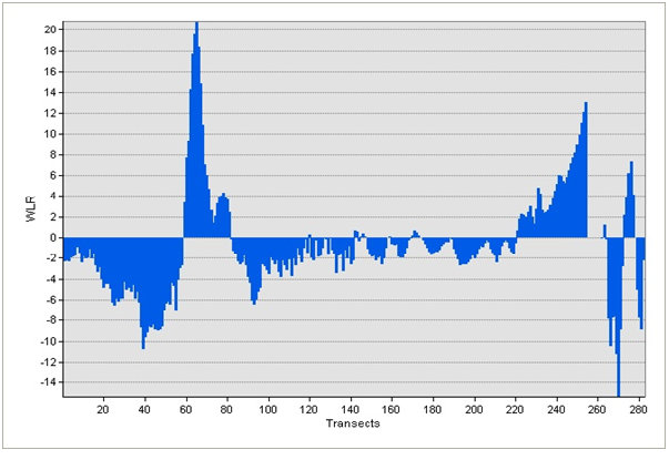
Shoreline change analysis provides important information upon which most coastal zone management and intervention policies rely. Such information is however mostly scarce for large and inaccessible shorelines largely due to expensive field work. This study investigated the reliability of medium resolution satellite imagery for mapping shoreline positions and for estimating historic rate of change. Both manual and semi-automatic shoreline extraction methods for multi-spectral satellite imageries were explored. Five shoreline positions were extracted for 1986, 1991, 2001, 2007 and 2011 covering a medium term of 25 years period. Rates of change statistics were calculated using the End Point Rate and Weighted Linear Regression methods. Approximately 283 transects were cast at simple right angles along the entire coast at 200m interval. Uncertainties were quantified for the shorelines ranging from ±4.1m to ±5.5m. The results show that the Keta shoreline is a highly dynamic feature with average rate of erosion estimated to be about 2m/year ±0.44m. Individual rates along some transect reach as high as 16m/year near the estuary and on the east of the Keta Sea Defence site. The study confirms earlier rates of erosion calculated for the area and also reveals the influence of the Keta Sea Defence Project on erosion along the eastern coast of Ghana. The research shows that shoreline change can be estimated using medium resolution satellite imagery.

Currently, coastal zones are facing intensified natural and anthropogenic disturbances including sea level rise, coastal erosion, over exploitation of resources among others. Over 70% of the world’s beaches are experiencing coastal erosion and this presents a serious hazard to many coastal regions (Appeaning Addo et al., 2008). According to Zhang (2010), awareness of the quality of global coastal ecosystems being adversely impacted by multiple driving forces has accelerated efforts to assess, monitor and mitigate coastal stressors. Monitoring temporal–spatial changes of coastal environments can help understand among others, the spatial distribution of erosion hazards, predicting their development trend and supporting the mechanism research on coastal erosion and its countermeasures.

For coastal zone monitoring, shoreline extraction in various times is a fundamental work. The shoreline, which is defined as the position of the land-water interface at one instant in time (Gens, 2010) is a highly dynamic feature and is an indicator for coastal erosion and accretion. The processes of erosion and accretion affect human life, cultivation and natural resources along the coast. Rapid shoreline changes can create catastrophic social and economic problems along populated strands. Design of viable land-use and protection strategies to reduce potential loss is necessary and this requires comprehension of regional shoreline dynamics (Blodget et al., 1991; Chu et al., 2006).

Shoreline changes occur over a wide range of time scales from geological to short lived extreme events (Appeaning-Addo, 2008). These changes are mainly associated with waves, tides, winds, periodic storms, sea-level change, and the geomorphic processes of erosion and accretion and human activities (Van and Bihn, 2008). While there is no doubt that shorelines are changing, the nature of changes is complex and the magnitude is uneven and vary from one point to another (Camfield and Morang, 1996). The detection and measurement of shoreline changes is therefore an important task in environmental monitoring and coastal zone management (Van and Bihn, 2008). According to Appeaning Addo (2008) historic shoreline change information, which portray a cumulative outcome of the processes that altered the shoreline for the periods analysed, facilitate formulating effective coastal management strategies and planning by revealing trends.

Remote sensing techniques provide a synoptic vision of the Earth that is not possible to obtain other than by exhaustive and expensive field evaluations. Data from remote sensors allow analysis of a region with sufficient accuracy in an efficient, rapid and low-cost way (Berlanga-Robles and Ruiz-Luna, 2002). It also helps in analysing areas that are poorly accessible or rapidly changing (Chu et al., 2006). The use of remote sensing data is therefore increasingly becoming a more effective option for monitoring shorelines. Over the years, geomorphologists, oceanographers and geologist have developed interpretation keys for mapping coastline geomorphic features using aerial photographs; however, few studies of this type have used images generated by remote sensing orbital instruments (Kawakubo, 2011). Though the use of aerial photographs tends to be effective in this case, the frequency of acquisition, cost and coverage presents a challenge. Furthermore, the spectral range of these sources is minimal and may introduce errors in shoreline interpretation (Alesheikh et al., 2007).

On the other hand, multispectral remote sensing satellites provide digital imagery in various spectral bands, including the near infrared where the land-water interface is well defined. Furthermore this approach has advantages: not time consuming, inexpensive to implement, large ground coverage, and the capability for repeat data acquisition and monitoring (Van and Bihn, 2008). The principal limitation of satellite images is arguably their low spatial resolution when compared to photographs taken from aircraft (Kawakubo, 2011).

1.1. Coastal Zone of Ghana

According to Armah and Amlalo (1998), Ghana’s coastal zone represents about 6.5% of the land area of the country, yet houses 25% of the nation’s population. This small strip of land now hosts 80% of the industrial establishments in Ghana. Over 70% of the shoreline of 550km is sandy (Armah and Amlalo, 1998). Coastal erosion, flooding and shoreline retreat are serious problems along the coast. According to Ly (1980) the eastern coast has been identified as the most erodible stretch with rates as high as 4m/year prior to the construction of the Akosombo Dam on the Rive r Volta. The construction of the Dam in the early 1960’s has supposedly reduced sediment supply to this coast offsetting the balance between the sediment lost to longshore drift and replenishment. Erosion rates increased reaching as high as 8m/year around 1970.

There have been interventions such as the Keta Sea Defence Project (KSDP) which involved stabilization of the shoreline with break water and groynes, construction of a flood control structure and land reclamation from the lagoon (GLDD, 2001). These among others have influenced the accretion and erosion patterns along this coast.

This paper explores the analysis of shoreline change using medium resolution satellite imagery including Landsat TM, Landsat ETM+ and ASTER imagery. The study spans over a period of 25years and covers the period before and after the construction of the KSDP. Erosion and accretion patterns are compared before and after the sea defence to determine the influence of the KSDP on rates.

2. Study Area

The coastal zone of Ghana is generally divided into three sections, the western, central and eastern based on the geomorphology (Ly, 1980) (Figure 1). The Eastern coast, which is about 149km, stretches from Aflao (Togo Border) in the East to the Laloi Lagoon west of Prampram. The shoreline studied covers about 52 km of this stretch, from the eastern side of the Volta estuary to Blekusu east of Keta. This shoreline generally falls within the Keta Municipality. The area falls roughly between latitudes 5^º25' and 6 ^º 20' North and between longitude 0 ^º 40' and 1 ^º 10' East. The landscape consists of a large shallow lagoon (Keta Lagoon complex) surrounded by marshy areas with a sandbar (sand spit) separating the lagoon from the Gulf of Guinea and a number of creeks along the coast. The sand spit is very narrow; barely more than 2.5km at its widest point with a general elevation up to 2m above mean sea level (Awadzi et al., 2008; Boateng 2009).

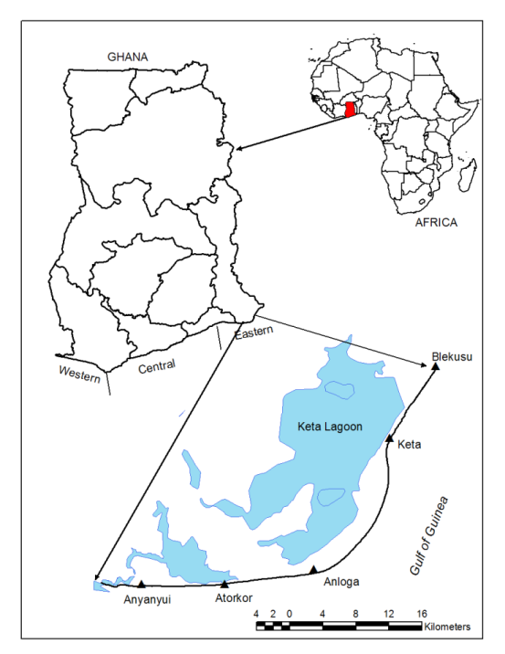Figure 1. Location of the Study Area (after Ly, 1980; Ghana Survey Department).

The geology of the area is soft and generally comprises quaternary rocks and unconsolidated sediments made up of clay, loose sand and gravel deposits (Akpati, 1978). The Volta River System, the main source of sediment supply to this basin, consists of a larger drainage basin, broad delta plain, narrow shelf, steep upper slope, and a large basin floor. Recent mapping of the sea bed topography reveals the presence of numerous canyons (valleys) from the shelf all the way to the deepwater (Manu et al., 2005).

Two types of wave approach this coast, the seas generated by the weak, local monsoon and the swell generated by storms in the southern part of the Atlantic Ocean. Average wave height for the area between 1997 and 2006 is 1.39m but may reach a height of about 3m. They normally arrive from the direction between south and south west with an average period of 10.91s which may reach a maximum of 19.68s (Svašek Hydraulics, 2006). Tides are semi-diurnal with an average range of about 1m. The tidal currents caused by this tides are weak.

3. Methods

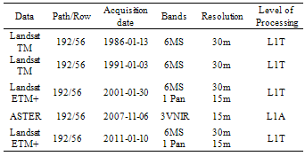
Four Landsat and ASTER imageries (Table 1) were used for analysing shoreline change. The imageries span a period of 25 years (1986, 1991, 2001, 2007 and 2011) and were acquired from the United States Geological Survey, Earth Resources Observation and Science Centre.

Table 1. Imagery Characteristics.

3.1. Data Processing

The Landsat TM data was resampled using nearest neighbour and 1^st order polynomial transformation to 15m. This however does not add any spatial information to the new data and increases the uncertainty for the shoreline position. For the Landsat ETM+ data, the panchromatic band with a resolution of 15m was used to sharpen the six multispectral bands to obtain a new image at 15m. The Gram-Schmidt pan sharpening algorithm in ENVI which is based on principal component analysis was used.

The ASTER VNIR bands were already at 15m but were acquired at L1A (raw data), hence the need for geometric correction/rectification. The VNIR bands were co-registered (Image to image) to the Landsat 2001 ETM+ data using 30 visually interpreted Ground Control Points (GCP). These GCPs were used to warp and resample the ASTER using first order polynomial and nearest neighbour transformation. The total root mean square (RMS) error was 0.35m.

3.2. Shoreline Extraction

The dry wet/boundary which approximates the high waterline (HWL) was extracted using semiautomatic and manual methods. Previous studies used the HWL as the shoreline proxy for change analysis in Ghana (Appeaning Addo et al., 2008; Appeaning Addo, 2009; Ly, 1980). Band ratio between the mid infrared (band 5 [b5]) and the green (band 2 [b2]) was used to identify the water-land boundary for the Landsat images except the 2011 image due to the gaps in the data. This was used so as to reduce the level of subjectivity in delineating the shoreline. For this study band ratio was implemented using the band ratio model in the ENVI software thus b5/b2.

The resulting image with ratio values between 0 and 3 was sliced and segmented to form a binary image with values less than 1 being classified as water and values greater than 1 being classified as land thereby delineating the boundary between the water and the land as the shoreline. The water class was then converted from raster to vector and exported as shapefiles for overlay in ArcMap.

In ArcMap, the extracted shorelines were overlaid on the Landsat image. The output vector however consisted of other water/land boundaries such as those of creeks and lagoons and could not be directly used for change detection. To extract the target sections, the extracted vector shoreline were overlaid on the colour composites and used as guide to digitize the target shoreline. The ASTER and Landsat ETM+ 2011 were however directly digitized.

3.3. Shoreline Analysis

The shoreline positions were compiled and managed in ArcGIS 9.3. A geodatabase was created for the extracted shoreline positions. Each shoreline has attributes which include date, length, ID, shape and uncertainty. The date of acquisition for each image was entered for the date column while the length, ID and shape were automatically generated. Uncertainties were also quantified and entered as integers for the uncertainty column. The five shoreline positions were then appended to one shapefile for rate calculation.

The Digital Shoreline Analysis System (DSAS 4.2) developed by the USGS in 2010 (Himmelstoss, 2009) was used was used for rate estimation. The software is an extension for ArcGIS and computes rate of change at user specified interval along the shoreline using different methods.

The DSAS uses measurement baseline method to calculate rate of change statistics for a time series of shorelines. The baseline is constructed to serve as the starting point for all transects cast by the DSAS application. For this analysis the baseline was constructed by manually digitizing about 500m onshore away from the closest shoreline, taking into consideration the general orientation of the shoreline.

Once all the inputs were ready in the database, transects were constructed. A total of 284 transects were cast along the entire stretch of shoreline from east to west at a specified interval of 200m. The transects were cast at simple right angles from the baseline. Historic rates of shoreline change were then calculated at each transect using end point rate (EPR) and weighted linear regression (WLR).

The EPR was employed where only two shoreline positions were available as was the case for the period between 2001 and 2007. The distance between the two points where the shoreline intercept a transect is calculated and this distance is divided by the number of years that have elapsed in this case 6years, to give the end point rate (equation 1) .

(1)

Where R₁ is the rate, Dm is the distance in meters between the two dates and T is the period between the two shoreline positions.

For the entire period under study five shoreline positions were available thus for 1986, 1991, 2001, 2007 and 2011 and uncertainties were also quantified (discussed below). WLR method was therefore used for calculating the rates. The method was also used to calculate changes for periods between 1986 and 2001 (period before the KSDP) and between 2001 and 2011 (the period during and after the KSDP). Both periods had three shoreline positions mapped. In computing WLR, more reliable data thus shoreline positions with smaller uncertainty, are given greater emphasis or weight towards determining a best-fit line. The slope of the regression line between the shoreline positions at each transect is reported as the change rate (equation 2).

(2)

Where y = distance from baseline; m = slope (rate of change) and b = y-intercept.

For this study, uncertainties were quantified using estimates based on studies such as Crowell et al. (1991) and Moore (2000) and Hapke et al., (2010). Additional errors, which were associated with the imagery used for this study, were estimated. Four main sources of error were identified to account for the uncertainties. Errors resulting from image registration, digitization of the shoreline, position of HWL and differences in resolution were considered. Resampling the 1986 and 1991 images from 30m to 15m did not add any spatial information but rather added to the uncertainty. An estimated error of ±3m is therefore assigned to the 1986 and 1991 shorelines.

The tidal range (1m) of the area was negligible and therefore was not accounted for as a source of uncertainty due the resolution of the imagery used. A total shoreline positional error for each epoch (E_x) was therefore calculated using the following equation:

(3)

Where E_s is the error occurring from scale difference, E_p is the photogrammetric error and E_r is the registration error. This approach carries the assumption that component errors are normally distributed (Dar and Dar, 2009).

The total uncertainties were used as weights in the shoreline change calculations. The values were annualised to provide error estimation for the shoreline change rate at any given transect and expressed as:

(4)

where E₁, E₂,... E₅ are the total shoreline position error for the various years and T is the 25 years period of analysis.

The maximum annualised uncertainty using best estimate for this study is ±0.44m/year.

4. Results and Discussions

A total of 7 shorelines were extracted from the satellites imageries and field work for shoreline analysis and accuracy assessment. The shoreline positions were for 1986, 1991, 2001, 2007, 2010 and two shoreline positions for 2011 as shown in Figure 2. The shoreline positions for 2011and 2007 had gaps.

Figure 2. Extracted Shorelines.

Change rates were calculated for the period between 1986 and 2007 and then for 1986 to 2011(Figure 3). This was to cross the check the effects of the gaps in the 2011 image on the rates. The results show that there have been significant changes along the entire coast for the 25 years period under study. For the period between 1986 and 2011, about 40% of transects were ignored due to the gap in the 2011 shoreline positions. This affected change rates especially near the estuary. However, overall rates show little variation when compared. The averages of the calculated rates are shown in Table 2.

Overall rates ranges from -12m/year to 18m/year where negative values represent erosion and positive values represent accretion (Figure 3). Using the 1986 to 2007 results as a reference, about 45% of the entire shoreline experienced erosion while the remaining have mostly accreted. No change was recorded for only one transect.

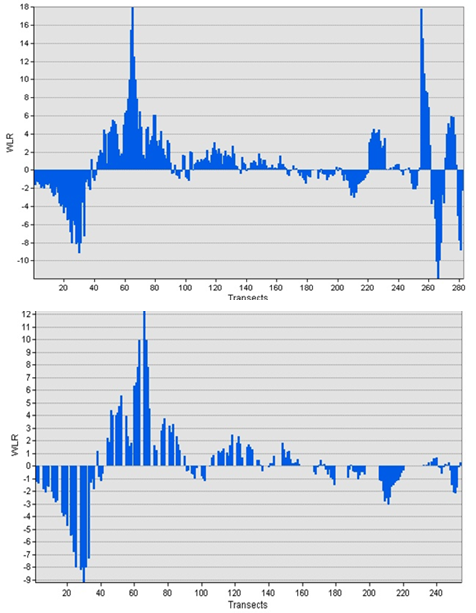Figure 3. Rates of Change (a) 1986-2007 and (b) 1986-2011.

Accretion rates range from 0.1m/year to 19m/year with an average 2.5m/year while erosion rates were between 0.1 to 9.3m/year with an average of 2.38m/year. Both rates are significantly high.

Table 2. Average Erosion and Accretion Rate.

The Keta area has seen much of accretion with rates reaching about 18m/year while the area between Keta and Blekusu has seen much erosion with rates at an average of 3.5m/year with some sections recording as high as 9m/year. Near the estuary there are extreme cases of erosion and accretion over the period and rates are as high as -11m/year and 17m/year respectively. For the entire shoreline erosion and accretion rates average at 2m/year.

The period before the KSDP (1986 to 2001) revealed that erosion dominates the entire shoreline (Figure 4) with about 70% of the cast transects recording erosion. Erosion rates range from 0.1 to 15.4 m/year with an average of 3m/year and accretion rates ranging from 0.1m/year to 21m/year with an average of 5.90m/year. The higher erosion rates occur between Keta and Blekusu and around Atorkor and Anyanui while the area between Keta and Anloga has experienced significant accretion. Close to the estuary there is evidence of both erosion and accretion over the period. Here erosion rates were as high as15m/year and accretion rates also at a high of 14m/year.

Figure 4. Erosion and Accretion Rates between 1986 and 2001.

Figure 5. Erosion and Accretion Rates (a) 2001-2007 (b) 2001-2011.

The period between 2001 and 2011 (after the KSDP) shows a reversal of situations with the entire coast experiencing more accretion (about 80%) (Figure 5). However, erosion rates have remained high ranging from 0.1 to 17m/year with an average as high as 4.5m/year. Accretion rates also were high ranging from 0.1 to 26m/year and an average of 5.6m/year. The area between Keta and Blekusu and the area near the estuary remain high points of erosion over this period with rates reaching as high as 16m/year.

It is also evident that most areas that experienced erosion between 1986 and 2001 have accreted between 2001 and 2007. The immediate vicinity of the Keta Township continues to accrete as well as areas around the estuary with values reaching 17m/year. Most portions of the Cape have also accreted.

4.1. Erosion Trends

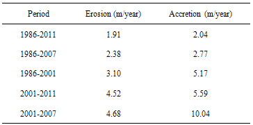
According to Ly (1980), erosion rates along the eastern coast have increased after the construction of the Akosombo Dam in 1962. The rates reached as high as 8m/year as compared to the 4m/year high rates before the construction. The result of this study reveals high rates of erosion along the entire coast for the period under study from 1986 to 2011 thus an average rate of about 2m/year ±0.44m. The period before the construction of the KSDP marked intense erosion along the entire coast with rates reaching as high as 15m/year and an average of about 3.10m/year for the area near Keta and the Volta estuary. This has led to destruction of many coastal facilities and homes especially at Keta. It also confirms the assertion that the Cape has been retreating since the construction of the Akosombo Dam (Boateng, 2009).

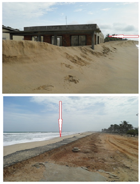Figure 6. Destruction by Erosion at (a) Blekusu and (b) Atorkor.

As part of efforts to curb the situation, the Keta Sea Defence project was initiated with work beginning in 2001. Thereafter, the rates indicate more accretion to the west of the site and erosion to the east. Erosion rates remain high averaging 4.52m/year while accretion rates were also as high as 5.5m/year. The high erosion rates in the east have led to the destruction of houses at Blekusu and its surrounding communities (Figure 6a). This situation confirms the knock-off effects by hard coastal protection measures.

Further down to the west (near the estuary) erosion rates had also increased leading to the destruction of homes and schools. As well the road linking Anyanui in the far west to Keta was completely cut off at Atorkor (Figure 6b). Efforts are underway to protect this area from further erosion.

Previous studies estimate erosion rates be 1.13m/year ±0.17 for the Accra shoreline (Appeaning et al., 2008) and Ly (1980) place estimates for the eastern coast between 4-8m/year. The current rates reflect this general trend.

4.2. Factors Influencing Erosion

4.2.1. Waves Currents and Tides

Waves are active in the study area and it is considered a high energy beach. The prevailing south-westerly wind causes an oblique wave approach to the shoreline. This wave approach generates an eastward littoral transport. Shoreline retreat is therefore due to removal of sand from the unconsolidated Quaternary sediments exposed at the shoreline to the littoral zone to compensate the sand loss caused by longshore transport. Since there are no major headlands to act as obstacles to the littoral transport rates of retreat along this coast is high (Ly, 1980; Boateng, 2009).

Furthermore, due to the generally sandy nature of the Keta beach, there is accelerated coastal erosion since mobile sand presents less resistance to wave action. The sand is easily removed from the coast and carried away by the drift.

According to Manu et al. (2005) recent mapping of the of the sea bed topography of the estuary area reveals the presence of numerous canyons (valleys) from the shelf all the way to the deep water. Waves at reaching this point may behave as in deep waters. The waves will therefore break at a higher speed on suddenly reaching the shoreline. The impact is stronger and may partly explain the high erosion rates along the Keta shoreline.

4.2.2. Construction of the Akosombo Dam

Sediment supply to the region from the Volta River is important. According to Ly (1980), prior to the construction of the Akosombo Dam sediment supply from the Volta River is estimated to be 71 million m³/a. This was carried along the wave-induced littoral drift to the east. In effect there was natural accretion at Cape St. Paul. With the construction of the Dam, this supply reduced to only 7 million m³/a leading to shortage of littoral sediment and hence reduction in accretion along the eastern strip since the late 1960s (Boateng, 2009). Accretion was now occurring further west of the Cape near the estuary (Atiteti) as a result of reduced ebb tidal energy from the Volta which is caused by the reduction of the flow of the river.

Further away from the estuary the shortage of sediment supply has led to the removal of sediments from the shoreline to compensate for this loss leading to increased erosion. Ly (1980) confirmed that this reduction led to an increase in erosion rates from an initial high of 4m/year to 8m/year. As confirmed by the results of this study, erosion dominates this shoreline prior to the construction of the Keta Sea Defence. The erosion rates have remained fairly high.

4.2.3. Sea Level Rise

Rising sea levels as a result of climate change are conspiring with coastal erosion to slowly submerge communities along the West African nation’s coast. Coastal systems react to changes in mean sea level by redistributing sediments. As supply of sediments reduce along this coast the shoreline retreats (Allersma and Tilsman, 1991). Keta has been identified as highly vulnerable to increased erosion associated with sea level rise (Boateng, 2009).

For the coast of Ghana, the local sea level is rising in conformity with the global trend at a historic rate of approximately 2 mm/yr. This is expected to increase, potentially up to as much as 6 mm/yr (Appeaning Addo, 2009). Higher sea levels exposes previously out of reach land to waves and currents increasing the vulnerability to erosion. This partially explains the high erosion rates found in this area. It has been identified that all the frontage of the Keta strip could be submerged by 1m rise in sea level, and 2m rise may result in inundation of the whole frontage (Boateng, 2009).

4.2.4. Shoreline Orientation

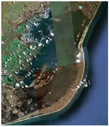Figure 7. The Shoreline Showing the Cape (Google Earth).

Cape St. Paul is a dominant feature along this coast projecting seaward and giving a convex shaped coastline. The shoreline roughly runs in the south-east direction (Figure 7). As sediments are supplied and transported from the Volta estuary greater part is deposited between its mouth and a point eastward of Cape St. Paul, where the littoral transport almost ceases. This is because the south–westerly waves cannot reach this area. Active erosion occurs here (point A, Figure 7); where the transport capacity increases and feeds the coast further east (Allersma and Tilsman, 1991).

This phenomenon is responsible for accretion around the Cape St. Paul prior to the construction of the Akosombo Dam. As discussed earlier, the construction of the Dam reduced sediment supply to this coast. The less sediment depletes quickly before reaching the Cape leading to the removal from the Cape onwards to compensate for the loss, hence the recession of the Cape after the construction of the Dam.

4.2.5. The Keta Sea Defence Project (KSDP)

As mentioned earlier, various attempts were made to halt the shoreline recession in the Keta area. The KSDP was the largest and was aimed at intercepting the reduced yet significant present littoral sediment drift (Boateng, 2009). The effect of this project on shoreline change was determined by comparing shoreline change before and after the construction. Prior to the construction of the Sea Defence, erosion was dominant along the entire coast especially around Keta.

With the completion of the project in 2004, erosion was greatly reduced as the shoreline between Keta and Havedzi was stabilized. There is the evidence of accretion along most sections of the coast especially west of the Defence between 2001 and 2007 as a result of the construction. However, the construction of site specific hard structures such as the Keta Sea Defence tends to stabilise a specific section of the coastline and cause a “knock on effect” down drift (Boateng, 2009). As confirmed by this study, to the immediate east of the Sea Defence erosion is occurring at high rates leading to the destruction of properties.

Furthermore there is increased erosion closer to the Volta estuary leading to massive destruction of coastal establishments. As part of efforts to curb the current situation, 2.5km long gabion revetment structure (Figure 8) is being constructed along the shoreline at Atorkor as well as the reconstruction of the road linking the community. About 500m of the revetment has been constructed and the rest will be completed by the end of the year 2011 (Ayivor, 2011). This is expected to stabilize the shoreline around this area but may shift focus to another point. There is the need for the development of SMPs for the management of Ghana’s shoreline.

4.2.6. The Land Squeeze Factor

Land use patterns have significant influence on erosion patterns. Increase in population along the coast puts much pressure on the natural land, making it more vulnerable to erosion. Rapid development along the coast of Ghana has been identified as a driving force for coastal erosion in Ghana. As discussed in section 3.8, land is, and remains a scarce commodity in the Keta area and as a result there high pressure on existing land. The sandbar on which the Townships are located is barely more than 2.5km at its widest point. The land is bounded in north by the Keta Lagoon and the south by the Gulf of Guinea.

According to Schleupner (2008), coastal development prevents coasts from adapting to increased erosion rates by shifting landward. Since the sandbar is limited in the north by the lagoon, developments cannot be moved further inland. As well, the land cannot adapt to sea level rise by migrating inland. In effect the available land is competed for by wave action as well as developments leading to squeeze situation. Furthermore, most of the settlements, historic and tourism sites and industries are within 200m radius from the shoreline.The impact of erosion is therefore felt in this area (Boateng 2006).

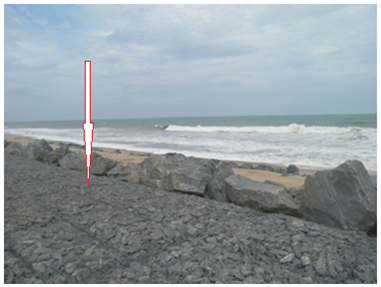Figure 8. Gabion Revetment Structure at Atorkor.

4.2.7. Sand mining and Mangrove Harvesting

Sand mining even though banned is being carried out in the area. Mensah (1997) has established that sand mining plays an important role in coastal erosion. The sand deposit ensures that sediment is available for littoral transport. Its removal reduces the beach volume and hence increases erosion. This has been identified as a major contributor to erosion along the Keta coast especially near Atorkor, Dzita, Dzelokope and Woe.

Also, mangroves prevent erosion by stabilising sediments with their tangled root system and also trapping sediments originating from inland thereby stabilising the shoreline. Over exploitation of mangroves has also been identified as a driving factor in increased coastal erosion. The intensified harvesting of red and white mangroves growing around Anyanui, Atorkor and Salo for domestics and commercial use has further aggravated the soil erosion problem (Keta Municipal Assembly, n.d.).

5. Conclusions

Results of this study have been useful in revealing the trends in shoreline change both erosion and accretion along the coast of Keta. Although aerial photographs are traditionally the main sources of data for shoreline monitoring, the study has shown that medium resolution multi-spectral satellite imagery can be used to map and monitor the large and dynamic shoreline of Keta. Though the study was only for the Keta coast, it is clear the methodology can be applied elsewhere.

Using the extracted shorelines, the DSAS was using in calculating the shoreline rate of change. The rates were calculated along transects that were cast along the entire shoreline using weighted linear regression. The findings generally confirm the high rates reported for this area after the construction of the Akosombo Dam. Average erosion rates are estimated to be 2m/year with the sections to the extreme east and west experiencing higher rates. The effect is the destruction of infrastructure along the coasts as evident at Atorkor and Anyanui. The second objective was hence achieved.

Natural factors including wave action, sea level rise and shoreline orientation are major contributors to shoreline change. The comparison of rates before and after the KSDP as discussed in section 6.2.5 has shown that, the structure is currently playing a major role in the erosion and accretion patterns in the area. Erosion is now taking place down drift (Blekusu and beyond). The shoreline around Keta and Cape St. Paul has been experience accretion since the completion of the KSDP. Other factors such as increasing pressure on the scarce land in the area, sand mining and mangrove harvesting in the area have been blamed for making the coast more vulnerable to erosion. The third objective has thus been achieved.

ACKNOWLEDGEMENTS

We are grateful to the USGS for making DSAS and satellite imagery available for this work. We also thank Scott Mitchell and Doug King of Geography and Environmental Studies Department, Carleton University, Canada for their contribution.