Mohammed Bennekrouf1, Zaki Sari2
1Depatrtment of Physics, Preparatory School of Sciences and Technology, Bel Horizon PoBox 165 RP, Tlemcen, 13000, Algeria
2Faculty of Technology, Manufacturing Engineering Laboratory, University of Tlemcen, PoBox 230, Tlemcen, 13000, Algeria
Correspondence to: Mohammed Bennekrouf, Depatrtment of Physics, Preparatory School of Sciences and Technology, Bel Horizon PoBox 165 RP, Tlemcen, 13000, Algeria.
| Email: |  |
Copyright © 2012 Scientific & Academic Publishing. All Rights Reserved.
Abstract
In the current design of reverse supply chain, several performance indicators must be considered and treated attentively. At this strategic level of the conception and to ensure a sustainable closed loop green supply chain, many qualitative as well quantitative criteria are taken into consideration with an environmental respect. Since the location allocation study persists as one of the most important area of research, we, in this paper propose a multi-objective multilevel green supply chain design. Firstly, we use an Analytical Hierarchic Process AHP multi-criteria approach to select the best sites for an eventual localization of remanufacturing center. Secondly, we formulate and solve a P median localization allocation model to manage the flow of mono-product in a dynamic closed loop supply chain. The proposed model is illustrated by several scenarios where environmental as well as economical interpretation is discussed.
Keywords:
Location-allocation, Closed Loop Supply Chain, AHP Approach, Mixed Integer Linear Programming
Cite this paper: Mohammed Bennekrouf, Zaki Sari, Multi-Objective Multi-Level Closed Loop Supply Chain Design, Management, Vol. 3 No. 5, 2013, pp. 266-272. doi: 10.5923/j.mm.20130305.04.
1. Introduction
With the increased environmental concerns and stringent environmental laws, reverse logistics has received growing attention throughout this decade. Remanufacturing is recognized as a main option of recovery in terms of its feasibility and benefits. However, little research has been devoted to the planning and optimization of direct and reverse logistic systems for network design. In the literature of closed loop supply chain, several works were discussed, in deterministic case. Assuming that recovery parts of product have the same properties as new parts, Zhou & al have examined both the direct and reverse recycling supply network which link between four partners: customers, distribution center, factories and recycling center[1]. Similarly, Lua & al have presented a two-level model under the code UNRM (Uncapacitated Remanufacturing Network Model)[2]. The model structure contains three types of plant to be located: the factory of production, remanufacturing center and intermediate center. Since the intermediate center regroups the activities of cleaning, disassembly, checking and sorting. The objective of their work was to minimize the number of plants to locate according to customer demand. In addition to that, it aims minimize the costs of operation, transportation and disposal (processes that occur at the remanufacturing and intermediate center). On other hand, for the remanufacture of several products, Lee & al have proposed m-RLNP (Multi level Reverse Logistic Network Problem)[3]. They minimize distribution costs (transportation) and open sites (disassembly center and processing) as well to reduce the complexity of their problem; the objective function is decomposed into three levels. The first level examines the management of the flow that occurs from the return center back to the center of disassembly. The second level deals with the management of reverse flow between the disassembly center and process center. Moreover, in dynamic closed loop supply chain approach, Tang and Xie have considered the environment protection[4]. For many products returned, several costs were integrated as transportation, inventory, operational, backorder and penalty. In addition to that, they have included the possibility of periodic opening or expending collection and repair facilities. Moreover, Min & al have proposed a two stages model were the return flow occurs from customers to centralized return center collection via collection center[5]. To ameliorate the quality of service under capacity constraints of collection center, the objective of their work was to search an optimal location of potential sites (collection center and CRC). Eventually, this is done in parallel to the minimization of several costs (inventory, rent, maintenance, installation and transportation). The benefit observed in this model is the inclusion of time as a variable in the objective function, in order to quantify the time of operation and periods of collection. In terms of service and economy and despite of the importance that brings the repair service for products returned under guarantee (Following a quality defect), a minority of works were interested in integrating the repair process in logistics of their origin supply chain. However, Min & al, have provided a reference case of study that takes into account the activity of repair[6]. Working in a dynamic multi-product environment, they propose a supply chain which contains three traditional entities (plant, distribution center, and customer) and repair center as a potential to ensure the recovery process. The objective of the proposed work is to find the optimal number and size of distribution and repair center to locate with taking into account the coordination between customers and plants.In addition, Pishvaee et al have examined the case of closed-loop supply chain network including customers at the first (reverse flow) and second markets (demand of returned product)[7]. Their problem of location aims to set up three basic elementary recoveries centers which are respectively, collection/inspection center, recovery center and redistribution between the two cited markets. To evaluate the uncertain of various input data, a set of agility indicator parameters was integrated during the calculation. To describe more a realistic case of study, these coefficients of agility can fluctuate the quantity of product returned from the first market, the customer demand in secondary market and the transportation costs between facilities.Otherwise Amin and Zhang have designed more complex closed loop supply chain with multiple plants (manufacturing and remanufacturing), demand markets, collection centres, and products[8]. Their goal of study is know how many and which plants and collection centres should be open, and which products and in which quantities should be stock in them. Two tests of problems are examined, first considering environmental factors including environmental friendly materials and second clean technology. To examine the effects of uncertain demand and return on the network configuration, a sensitivity analyses by scenario is used to minimize the total cost were tow approach of resolution was compared weighted sums and ε-constraint methods.For a market where a requests vary by a wide margin, the work of Zeballos et al is dedicated to the problem of the design and planning of closed-loop supply chains in that the number and location of the different types of network entities should be determined over the complete planning horizon[9]. These entities are factories, warehouses, customers, and sorting centers. For the operational level two time scales the planning are required: the demand and return values must be satisfied in macro-times (for instance, yearly), while supply, production, transportation, storage an collection values must be determined in micro-times (for instance, monthly). The problem goal is the total supply chain profit maximization in the case of multiple products flow under demand satisfaction were new and recycled products are indistinguishable and limited capacity of cited facilities. More than return levels is uncertain with several quality grades at the sorting centers. The formulation relevance was evaluated by an example based on an industrial case that involves the closed loop supply chain of a Portuguese glass firm.Also the work developed by Lee et al in several stages, presents one of more distinctive works which concerns the design of global logistics network in dynamic and stochastic approaches[10]. To provide more flexibility to the chain, the authors have implemented in the design a new entity called Hybrid Processing center. Depending on need and timing of demand, the role of HPC is to transfer from a distribution center to a collection center or the opposite. As for making decisions related to the choice of network configuration, the capacity of the three intermediate centers deposit (distribution, collection and HPF) must be adjusted shrewdly for optimal response to the command. Moreover, in the stochastic case, the use of vector representation of the model becomes inevitable combined with a probability function, thus defining the possible scenarios depending on uncertain parameters. In the both cases (dynamic or stochastic) the approach of the resolution used is SAA (Sample Average Approximation) hybridized with SA (simulated annealing: used to make the coding domain of the feasibility region of localization).In this paper, we study closed loop recovery network. The proposed model represents an extension of work Bennekrouf & al[11]. To manage the potential site of recovery through remanufacture, firstly we use AHP method. Therefore P median localization allocation problem is developed in the case of dynamic capacitate tow levels system with six entities as shown bellow in figure 1.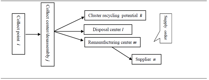 | Figure 1. Supply Chain Configuration |
2. Study Methodology
A. Quantitative ApproachIn the current selection of remanufacturing potential sites, numerous criteria may be considered when thinking about the best plantation. Qualitative as quantitative were weighted crucially to give a complicate multi-objective judgment. The alternatives considered in this study are: direct cost, social impact, logistic potential and life cycle of reuse modules. The weight measurement fluctuates among 1 and 9. B. Closed Loop Chain DesignThe For multi objective oriented cost decision making, the proposed model is subdivided in tow levels. The first level ensures the physical flow supplying from collection points to collection/dismantling center. After dismantling, testing then the storage of modules throughout a period T, in the second level several appropriate selective deliveries and treatment occur from selected collection/dismantling center to the set of recycling center, remanufacturing center then disposal center. Since the capacity of remanufacturing centre is limited, the remainder of entreats remanufacturing modules must be shipped to disposal center. This flow occurs in the case when the potential of opened remanufacturing center can’t cover all returned remanufacturing modules.C. Model FormulationSets and index , index of collection points (which can represent customers or retailers),
 , index of collection/dismantling center,
  , index of recycling cluster center,
 , index of disposal center,
  , index of potential location for remanufacturing center
 , index of supplier,
 , index of remanufacturing modules,, index of time periods,The parameters, variables and formulation of the problem are presented as:First level location-allocation formulation The parameters of the problem are the following:
  fixing cost to install collection center at the site j (setting up & operating),
 : minimum capacity of collection center j,
 maximum capacity of collection center j,
 : distance between entities i and j in km,For product the parameters notations are:
 : transportation cost per km per kg
 real quantity of product collected from collect point i during time period t,
 : maximum quantity of product collected from collect point i during time period t,
  average size of product in m3,W: average weight of product in kg,Opc: operational cost related to the disassembly of product The decision variables for the first model are as follows:
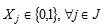
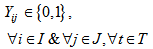
 : =1, if a collection center is located and set up at potential site j 0, otherwise, Yij=1, if collection point i is assigned to collection center j, 0 otherwise, The first level objective function Z1 minimizes investment cost and the best flow shipment from collection point to opened collection center is:
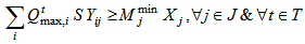
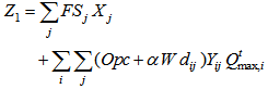 | (1) |
s.t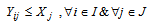 | (2) |
 | (3) |
 | (4) |
 | (5) |
 | (6) |
 | (7) |
Let  volume of product p shipped from all collection point i to collection center j during time period t defined as:
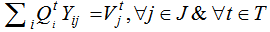 | (8) |
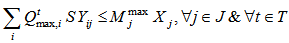
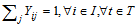
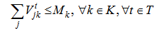
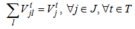
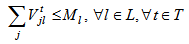
The constraint (2) assigns the physical flow from collection point i to collection center j located at node j. The constraint (3-4) forces each demand node i to be served by node j under capacity. Constraints 5-6 checks for binary variables and constraint (7) ensure that only one collection center is connected to collection point. As result to be used in second level, the equation (8) defines the real quantity of product collected in collection center j during the period t.Second level p-median location-allocation formulationThe parameters and variables of the problem are: : distance between entity
  and
and  in km: transportation cost per km per kg in the second level• Parameters and decision variables linked to the recycling clustering center kWk: average weight of recycling part of productMk: recycling clustering center k capacityPcostk: average profit cost of recycling part
 volume of recycling part of product shipped from collection/disassembly center j to recycling clustering center k during the period t+1• Parameters and decision variables linked to disposal center lWl: average weight of disposal part of productMl: disposal center l capacityPNcostl: penality cost to eliminate a disposal part of product at disposal center l
 volume of disposal part of product shipped from collection/disassembly center j to disposal center l during the period t+1• Parameters and decision variables linked to remanufacturing center mWr: average weight of each remanufacturing module rfr: average fraction of each remanufacturing module r specified as good to sale to suppliers nwldrm: workload required to treat module r in remanufacturing center mOPcostrm: operational cost to treat remanufacturing module r in remanufacturing center mWld_totm: workload total available at remanufacturing center mFSm: fixed cost to establish remanufacturing center at site mPNcostrm: penalty cost to eliminate bad remanufacturing module rin remanufacturing center m (assuming the existence of elimination task which is concern (1-fr) quantity)
 volume of bad remanufacturing r shipped from collection/disassembly center j to remanufacturing center m and then eliminated during the period t+1
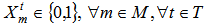
 if remanufacturing center m is located and set up at potential site m in period t+1, 0 otherwise,
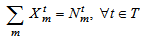
  : number of opened remanufacturing center m in time period t+1• Parameters and decision variables linked to supplier n
 : unitary supplier n demand of remanufacturing module rPcostrn: unitary average remanufacturing module profit cost for supplier n
 volume of remanufacturing module r shipped from collection/disassembly center j to supplier n via remanufacturing center m during the period t+1. • Parameters and decision variables linked to dispose remanufacturing module r at disposal center lWld_totl: workload total available at disposal center l to eliminate any remanufacturing module r (this operation occurs when the capacity of remanufacturing network can’t recover collected remanufacturing module r) wldrl: workload required to eliminate module r in disposal centerlPNcostrl: penalty cost to eliminate remanufacturing module r in disposal center l
 volume of eliminated remanufacturing module r shipped from collection/disassembly center j to disposal center l during the period t+1The second level location-allocation problem consists to minimize various costs where the objective function Z2 is:
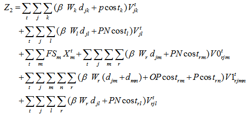 | (9) |
s.t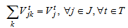 | (10) |
 | (11) |
 | (12) |
 | (13) |
 | (14) |
 | (15) |
 | (16) |
 | (17) |
 | (18) |
 | (19) |
 | (20) |
 | (21) |
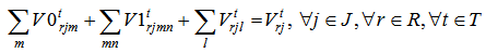
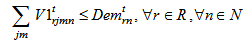
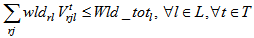
The fixed costs are linked to the opening manufacturing center. The variable costs includes transportation costs, operating costs and benefits at recycling clustering center, remanufacturing center and suppliers as well as penalty costs of elimination at disposal center and remanufacturing center. Equations (10-11-12-13) equilibrate the capacitate supply flow of recycling parts to recycling clustering center, and disposal parts to disposal center. The set of constraints (14-15-16) defines the quantity of remanufacturing modules that are shipped from collection/disassembly center to suppliers via remanufacturing center with respect to their qualities defined by the fraction and the capacities of remanufacturing center. The equations in constraints (17-18) guarantee the shipment limit of remanufacturing modules to suppliers with the respect to the capacities and demands parameters. Inequalities (19) ensure that the remainder of entreats remanufacturing modules must be shipped to disposal center. The constraint (20) imposes binary conditions and condition (21) gives the number of remanufacturing center that can be opened
3. Numerical Computation
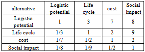
The selection of remanufacturing center is based upon the classifying of four alternatives with a weight see Table 1. For logistic potential criteria; means the physical transportation links plus the commodities of storage and delivery. About the second alternative that presents live cycle after reuse of modules is the most important as parameter of sustainability and environment. Their consideration selects the nearest green suppliers to candidate potential remanufacturing center. For the cost alternative is estimated relatively to cost of implantation and transportation cost. Where the latest alternative; social impact is evaluated after a list of questions to the person which are neighbor to the candidate remanufacturing site. The questions are focused on the environment and ergonomic impact. After the normalization of AHP matrix, we have selected four sites among ten.Table 1. Alternative Comparison Matrix
 |
| |
|
The study was applied in area of 1000 km2, where the chosen geometrical configuration of supply network is illustrated in figure 2. To describe the problem, we assume that twenty collect points want to construct the recovery logistics network. The first shipment occurs from the collect points to six candidate’s collect/disassembly center facilities with limited capacities of storage per unit of volume. After calculation, the reverse procurement occurs from only four opened collect/disassembly center to their nearest recycling cluster potential and disposal center with unlimited capacity. Furthermore, the good quality of remanufacturing modules is shipped to the supplier via remanufacturing center. The recovery rate of remanufacturing received modules by scenario gives the environmental interpretation as it mentioned in Table 2. Because the cost to set up the remanufacturing center is in the responsibility of authorities and original manufacturing, their investment should be progressive.In consequence it more appropriate to install thus potential facility during a planning horizon. For example in each year, only one remanufacturing center is opened.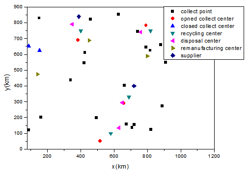 | Figure 2. Supply Chain Configuration |
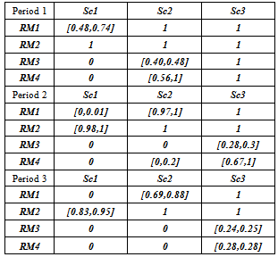
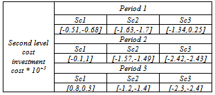
The table 2 summarizes the variation interval of recovery rate of each module by scenario and by period (each period has a longer of four month).In limit it appears that when three remanufacturing centers are operational, for modules three and four, the recovery rate does not reach 100% in the period three. But if additional hours will be added the problem will be solved. Also in Table 3 the economic interest is visualized as a benefit for all scenarios except scenario 1 in period three.Table 2. Recovery rate of remanufacturing moduls RM per scenario (sc) and per period (%)
 |
| |
|
Table 3. Second level investment cost per scenario
 |
| |
|
4. Conclusions
Reverse logistics is still a new research field, although a lot of achievements have been made in recent years. In this paper, we have presented a closed loop logistics network design and planning in dynamic approach. Before the study of quantitative location allocation problem, we have used the qualitative AHP approach to select the best eventual geographical sites to locate remanufacturing center. Therefore, MILP programming model is proposed and validated by lingo 12 solver. The mathematical proposed model aims to select the best appropriate sites for the opening of collection center as remanufacturing center. Further, the quantity and quality of remanufacturing modules was considered to optimize location and the allocation of physical flow. Also, an analysis per scenario was given to illustrate the progressive recovery rate since reverse logistic network is done in multi firm collaboration. Our contribution is to facilitate the treatment of primary closed loop supply chain. As perspective, it is more important to add others parameters as inventory between the period and others recoveries factories.
Appendix
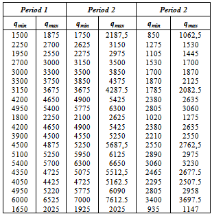
Table 4. Returned Quantity in each collect point per period
 |
| |
|
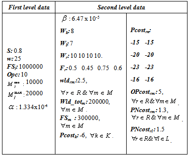
Table 5. Second Level & First Level Data In Unity Of Mesure
 |
| |
|
References
| [1] | Y.S. Zhou, S.Y. Wang, “Generic model of reverse logistics network design,” Journal of Transportation Systems Engineering and Information Technology, vol. 8(3), pp. 71-78 (2008). |
| [2] | Z. Lua, N. Bostel, “A facility location model for logistics systems including reverse flows: the case of remanufacturing activities,” Computers & Operations Research, vol. 34, pp. 299-323 (2007). |
| [3] | D. Lee, M. Dong, “Dynamic network design for reverse logistics operations under uncertainty,” Transportation Reasearch Part E, vol. 45, pp. 61-71 (2009). |
| [4] | Q. Tang, F. Xie, “A Genetic Algorithm for Reverse Logistic Network Design,” IEEE Third International Conference on Naturel Computaion, (2007). |
| [5] | Min, H., Ko, Y. J.: The dynamic design of a reverse logistics network from the perspective of third-party logistics service providers, International Journal in Production and Economics, vol. 113, pp. 176-192 (2008). |
| [6] | H. Min, Y. Ko, C. S. Ko, “A genetic Algorithm approach to developing the multi-echelon reverse logistics network for product returns,” The International Journal of Management Science, vol. 34, pp. 56-69. Omega (2006). |
| [7] | M. S. Pishvaee, M. Rabbani & S. A. Torabi, “A robust optimization approach to closed-loop supply chain network design under uncertainty,” Applied Mathematical Modelling Computers, vol. 35(2), pp. 637-649 (2011). |
| [8] | S. H. Amin,G. Zhang, “A multi-objective facility location model for closed-loop supply chain network under uncertain demand and return,” Applied Mathematical Modelling, vol. 37(6), pp. 4167-4176 (2013). |
| [9] | L. J. Zeballos, M. I. Gomez, A. P. Parbosa-Pavoa, A. Q. Novais,” Addressing the uncertain quality and quantity of returns in closed-loop supply chains,” Computers & Chemical Engineering, vol. 47, pp. 237-247 (2012). |
| [10] | D-H. Lee, M. Dong, W. Bian, “The design of sustainable logistics network under uncertainty,” International Journal of Production Economics, vol. 168(1), pp. 159-166 (2010). |
| [11] | M. Bennekrouf, W. Mtalaa, F. Boudahri, Z. Sari, “A Dynamic Model for the Design of Green Logistic Networks,” 41 Conference in Computers and Industrial Engineering, Los Angles (2011). |
 Abstract
 Reference
 Full-Text PDF
 Full-text HTML