-
Paper Information
- Next Paper
- Previous Paper
- Paper Submission
-
Journal Information
- About This Journal
- Editorial Board
- Current Issue
- Archive
- Author Guidelines
- Contact Us
Management
p-ISSN: 2162-9374 e-ISSN: 2162-8416
2013; 3(4): 206-217
doi:10.5923/j.mm.20130304.03
A Mechanism for Determining Tanker Truck Transport Rates: A Case of Oil Products Supply Chain
 Abstract
 Reference
 Full-Text PDF
 Full-text HTML
Mostafa Mousavi1, Mohammad Bakhshayeshi Baygi2, Elnaz Miandoabchi3, Narin Asgari4, Reza Zanjirani Farahani5
1Ecole Polytechnique, Palaiseau, Paris, France
2Mechanical and Industrial Engineering Department, University of Concordia, Montreal, Canada
3Logistics and Supply Chain Research Group, Institute for Trade Studies and Research (ITSR), Tehran, Iran
4Logistics and Management Mathematics, Department of Mathematics, University of Portsmouth, The UK
5Kingston Business School, Kingston University, Kingston Hill, Kingston Upon Thames, Surrey KT2 7LB, The UK
Correspondence to: Narin Asgari, Logistics and Management Mathematics, Department of Mathematics, University of Portsmouth, The UK.
| Email: |  |
Copyright © 2012 Scientific & Academic Publishing. All Rights Reserved.
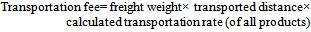
In order to minimize costs of an oil products distribution company, it is important to determine the appropriate transport rates (TRs) that lead to satisfying both the transporters and the company. This paper introduces a systematic and scientific method for calculating the TRs for tanker trucks. Calculating TRs is based on a combination of finished cost and engineering economics techniques in which all the costs related to the tanker truck transportation are considered as financial flows over time. Finally, we explain about designing a computer-based system for calculating the TRs and estimating the required budget.
Keywords: Freight Transportation, Oil Products, Transportation Cost, Tanker Truck
Cite this paper: Mostafa Mousavi, Mohammad Bakhshayeshi Baygi, Elnaz Miandoabchi, Narin Asgari, Reza Zanjirani Farahani, A Mechanism for Determining Tanker Truck Transport Rates: A Case of Oil Products Supply Chain, Management, Vol. 3 No. 4, 2013, pp. 206-217. doi: 10.5923/j.mm.20130304.03.
Article Outline
1. Introduction
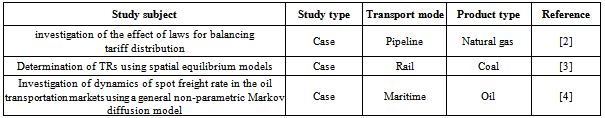
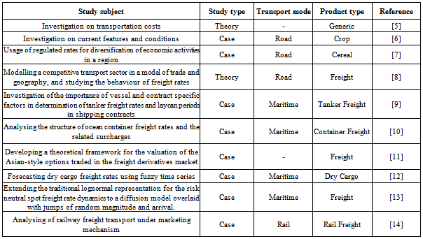
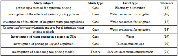
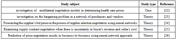
- One of the main goals of NIOPDC is the distribution of oil products across the country. Transportation costs constitute 60 percent of companies’ current costs [1]. Therefore, determining appropriate TRs is crucial in order to satisfy both the third party transporters and the company. Currently, in the company, determination of TRs is undertaken by experts. This task is very time consuming and the resulted rates may not be satisfactory in some cases by transport companies. Oil products transportation is important for today’s conditions of the country due to increasing demands for this precious substance. Therefore we develop a mechanized system for estimating the TRs and the annual needed budget. The company can apply the adjusted rates directly or account on them as a reliable basis for further negotiation with transport companies, because our estimations are based on logical inferences.Generally, in the related literature, there are two main techniques used in TRs estimation: First, a financial and accounting method, in which TRs are estimated according to the total transportation cost which adds up transportation costs and profit of the transporters; The second is based upon microeconomic concepts and equivalence between supply and demand in which a trade-off is made between supply, demand and price of product or service. In general, the studies in TRs determination are classified into a number of categories. Table (1) depicts a summary of the transportation rate literature for fuels (e.g. oil, coal and gas), Table (2) summarizes the transportation rate literature for non-oil freight or generic freight, Table (3) demonstrates a summary of the tariff determination literature and Table (4) shows a summary of the negotiation literature.In this paper a scientific and logical algorithm is designed so as to calculate the oil products TRs for oil and gas tanker trucks. Finally, a mechanized system is used for calculating the TRs and estimating the required annual transportation budget. It is important to emphasize that we have combined both "finished cost" and "time value of money" concepts in order to design the algorithm and develop the mechanized system. The remainder of the paper is organized as follows. Section 2 is the status quo which is a description of current oil products supply chain, and then it reviews what is now happening to calculate the TRs in the company. Section 3 states the case problem (its goals, scope, inputs, outputs, etc) in details. Section 4 proposes the developed system and explains the approaches and techniques which should be used to calculate the TRs. An example is illustrated in section 5. In section 6, all necessary input data for calculating the rates are mentioned. The results are shown in section 7. In addition, we have performed a sensitivity analysis on the input data to see how precise we have to be in gathering data as input. Finally section 8 is the conclusion.
|
|
|
|
2. Status Quo
- As shown in Figure 1, the supply chain of oil products in the country has four tiers: a) origins including refineries, coastal origins and ports which are used for liquid fuel importation, b) main national depots, c) secondary domestic depots, and d) customers or retailers like fuel stations and large industries; naturally end-consumers will be positioned in customers downstream. Based on districting pattern at NIOPDC, the country can be divided into a number of zones from the perspective of oil products supplying operations. Each zone itself has at least one depot in order to meet its demands. Tanker trucks, in six wheels, ten wheels and eighteen wheels (trailer type) are the modes used for oil products transportation in order to carry products from one depot to another depot or to retailers. Different road conditions in terms of coverings, geographical conditions, and traffic, affect transportation costs. Our developed pricing mechanism estimates the TRs in advance while taking into account the diverse conditions and subsequently different costs that a tanker truck will have in the origin, road and destination.
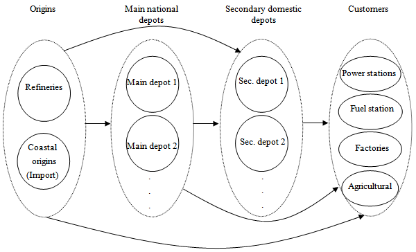 | Figure 1. Tire scheme of oil products supply chain |
2.1. Oil Products Supply Chain
- Oil products supply chain consists of 4 tiers. The products do not necessarily get involved in all tiers and it is even possible that they move between fixed entities within a tier. Figure 1 illustrates the flow of the oil products between and within the tiers. It is worthwhile to mention that procurement and secondary depots are almost similar and the only difference between them is in their capacity and level of equipments.• All depots regardless of being main or secondary are called procurement depots.• There are nine depots near the refinery which are fed through pipes from there. There are also a few depots near coastal origins and products flow into them when there is no load.• Currently, the company divides the country into a number of regions and each of them is in charge of supplying and distributing its own fuel and all other corresponding operations. Furthermore, every region is divided into a number of sub-regions and one of them is chosen as the central one.• Each region has at least one depot but not all the sub-regions necessarily have one. Central depots are independent of the sub-region and are managed by the region authorities.• The product is usually transported from a primary depot to other depots and then is distributed among consumers and retailers. In the sub-regions which do not have their own depot, the consumers and retailers are directly fed from the region depot.• Products are loaded in the origins and without any unloading during their route and in the other regions, are directly unloaded in the destinations.
2.2. Previous Systems
- In this section, the similar systems which had been used by the company for determining the TRs are discussed.
2.2.1. Earlier TRs Determination
- In the past, the base of transportation rate determination process was the linear regression formula Y=a+b.x. In order to estimate the transportation rate of crucialroutes, coefficients f1, f2,..., f6 were defined which play the modification role.
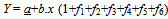 | (1) |
2.2.2. Current TRs Determination Classifications
- So far, the TRs and tanker trucks fees are calculated according to two rates: exempt and tariff TRs and basic and special TRs.
2.2.2.1. Exempt and tariff TRs
- This kind of classification is based upon the ownership of the transportation fleet. Exempt TRs are used for the calculation of exempt transportation fleet fees. Exempt fees are used according to the operational necessities, geographical circumstances and time and location constraints and are determined via the experiences of experts, data gathered from different resources and field studies.Tariff rates are used for the calculation of under contract transportation fleet. Most of under contract transportation is allocated to various regions by contracts. There are two kinds of under contract transportation: Outsourced and In-sourced fleet.• Outsourced fleetThis fleet is the kind in which the tanker truck is rented by the drivers for a specific time and during this period; the company is the owner of the tanker truck.• In-sourced fleetThe ownership of this fleet is personal or corporative. Tariff Rates themselves are divided into two categories according to a given delivery radius: Urban TRs and Procurement TRs.Urban TRs are calculated for the transportation within the urban radius. Urban radius is the distance determined for any city according to its geographical and topological conditions. Urban transportation rate unit is Rials per litre and the fee is calculated according to the beneath equation:
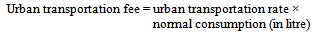 | (2) |
 | (3) |
 | (4) |
2.2.2.2. Basic and Special TRs
- These rates are determined according to the delivered products. Basic TR includes diesel, solvents, lubricants and basic engine oils. While, special TRs are related to the transportation rate of products with special features like high inflammable materials and materials which have problems in loading and unloading. For such products TR is 10% more than the TR of the other products. These products include aviations fuels, premium gasoline, engine oil, gasoline solvents including JP4, AW, and furnace fuel.
3. Case Problem
- In this section, the problem features including its assumptions, objectives, constraints, inputs and outputs are discussed. In this problem, there are some important assumptions:• Supply chain of oil products consists of four tiers: refineries and crude oil ports, main national depots, secondary domestic depots, and fuel retailers (vendors, corporations, and main consumers)• Distribution company has divided the country into a number of zones and each one is responsible for fuel supplying, delivery and other related operations in the its own district. Besides, every zone consists of a number of areas.• Oil products are transported by four modes: pipelines, tanker trucks, rail and ships.• Every depot has a defined zone in which the transportation rate is calculated according to the load volume in terms of transported fuel which is measured in Litres. Outside of the zone, transported fuel is measured in tons.• Oil tanker trucks are in six wheels with the capacity of 6 to 14 thousand litres, ten wheels with the capacity of 14 to 20.5 thousand litres and trailer type with the capacity of 24 to 36 thousand litres.• Tanker trucks carrying natural gas are usually 18-wheel tanker trucks and their tanks are completely different from the oil ones.• The country’s transportation system features, including road, regional and climate conditions, road covering and safety, type of load and related dangers are different in various routes.The main problem objectives are:• Calculation of the oil transportation rate based on logical inferences (including base and adjusted rates) to achieve a reliable base for further negotiation• Development of a mechanized system to estimate the TRs and its total budgetScope of the problem is:• The Problem includes wide range of oil products; the main products are kerosene, gas oil, fuel oil, and motor gasoline. Natural gas is transported in the country using two transportation modes: tanker truck which lies in the scope of this research and pipeline which is out of this scope. For more information on the pipeline supply chain network, interested readers are referred to [27].• The problem includes all routes that are used for transporting with an amount of fee.• Different types of tanker trucks are included in the scope.This problem needs these inputs:• List of oil products and their features• List of all oil sources and destinations including fuel depots and retailers• All transportation routes features like route length,topography, climate conditions, road covering and traffic type.• All cost items necessary to calculate the transportation rate• The previous year information about (the) oil products transportationThe problem has to achieve these outputs:• A user-friendly piece of software to calculate the base and the adjusted rates for various types of oil products in every month of the year, considering different types of tanker trucks.• A user-friendly piece of software to estimate the annual budgets for oil products procurement and urban transportation
4. Developed System
- In this section, the designed approach and technique for calculating the TRs is presented and then the developed software for TRs calculation and budget estimation is introduced.
4.1. Two Generic Approaches for the TRs Determination
- Among the two generic approaches for determining the transportation rate, only one is selected here. First one is based on learning from previous patterns and behaviors while the foundation of the latter is based upon the total transportation cost.In the first approach, relying on the past proper made decisions and behaviors, a model is designed to determine the weights of the related factors in the transportation rate while taking into account these weights and factors and current or future situations. These models analyze previous applied rates and their relevant factors and employ forecasts and estimations techniques for the process of determination. In spite of the first approach that relies on the past behaviors, the second one, called total transportation cost which is used in this paper, estimates the total transportation cost while taking into account the time value of the money. This approach also assumes that there is no logical or scientific pattern in the previous cost estimations.
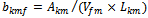
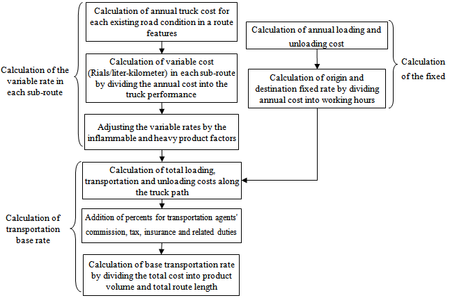
4.2. Designed Techniques for TRs Determination
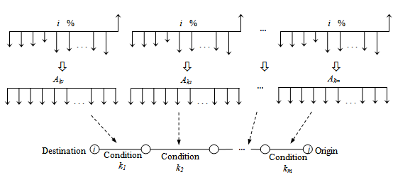 | Figure 2. Procedure for calculating the unit transportation cost throughout a route |
4.2.1. Variable Transportation Rate Cost Calculation of Each Sub-route
- Since different tanker trucks have different costs during the time, their financial flow varies from one to another. In order to consider the effects of temperature on cost items and also transportation conditions for every product, unit cost is calculated for each sub-route, tanker truck and product type. For calculating the transportation rate for each month of the year, the tanker truck, sub-route, product type and interest rate are shown in m, k, f and i, respectively. Then, the following procedure is applied to calculate the TRs:Step 1. Current value (in Rials), Pkm, of repetitive costs, A'km, with Tkm repetition frequency is calculated for the sub-route with features k and the tanker truck m according to equation (5).
 | (5) |
 | (6) |
 | (7) |
4.2.2. Fixed Loading and Unloading Costs Calculation
- For calculating the fixed loading and unloading costs, all of the tanker truck costs in the financial flow that do not have any relationship with its performance are considered and the EUAC for each tanker truck type,
 , is computed. Then by determining the total tanker truck work hours, h, and loading and unloading times, t, the loading and unloading costs, aij, are calculated according to equation (8). ai and aj are the loading and unloading costs at the origin and destination.
 | (8) |
4.2.3. TRs of Each Product Type
- Considering the fixed and unadjusted base rate given, the transportation rate of each product type in every month of the year by all kinds of tanker trucks could be calculated. The total transportation cost of a product from an origin to a destination is the sum of fixed loading and unloading costs and all variable costs through the route. The total transportation cost (in Rials) from the origin i to destination j have been shown in TCij and is calculated by the equation (9):
 | (9) |
 is the adjusted transportation cost and Ifm is the insurance cost of product f, if it is carried by tanker truck m. At last, some costs including tax, insurance, duties associated with the act of transportation between two cities, and commission of transportation agents are added by the parameter c. Base transportation rate from i to j, rij, is calculated according to equation (10). Unit of rij in urban areas is Rials per liter-kilometer, and in non-urban areas is Rials per ton-kilometer.
 | (10) |
 | Figure 3. Flowchart of base rate calculation model |
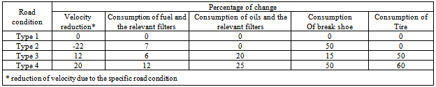
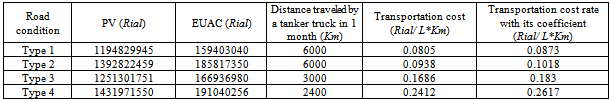
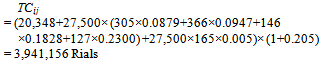
4.3. An Example
- In order to show how the procedure works, an example is presented in this section. The route under study is between an origin depot near the city of Abadan and the destination depot of Ray (a county of Tehran). The transported commodity is kerosene, the truck is trailer and the chosen month is May. The sub-routes of the interested route have four different conditions including (1) asphalted, flat, mild temperature, normal traffic (2) asphalted, flat, warm temperature, normal traffic (3) asphalted, hilly, average temperature, normal traffic (4) asphalted, mountainous, mild temperature, normal traffic. For each condition, the transportation costs are calculated. Table (5) illustrates change percentage in truck performance and consumption rate of items for each condition. The first road is considered as baseline condition.
|
|
 | (11) |
 | (12) |
4.4. Budget Estimation
- In this section, the method for estimating next year transportation budget according to the calculated rates is explained. The next year transportation budget is estimated on the basis of information from the previous years, because the monthly depot to depot transportation is estimated only for the next month. Budget estimation consists of procurement transportation (depot to depot transportation) budget and depot to retailers transportation budget. The method for calculating each part of the budget is interpreted:
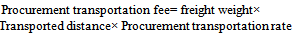
4.4.1. Procurement Transportation Budget
- Because procurement transportation includes most of the annual transportation budget, it is estimated by considering the transportation between each depot to has enough accuracy.If the litres of transported product f in month t of the previous year from origin i to destination j by oil tanker truck m is shown by
 , its calculated transportation rate in Rials per liter-kilometer is denoted by
  and finally the demands growth rate in the related region is denoted by
 , then the total procurement transportation budget is calculated by equation (13):
 | (13) |
4.4.2. Depot to Retailer Transportation Budget
- Considering the large number of retailers all over the country and consequently large amount of information obtained from them, the following formula (in which enough level of accuracy is tried to be maintained) is proposed for calculation of depot to retailer transportation budget:
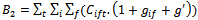 | (14) |
 and
and  are the total costs for transporting product f from the origin i to retailers in month t, the demand growth rate of product f in region i and inflation rate, respectively.
4.5. Designed System
- In this section, the designed system which supports the models of rate calculation and transportation budget estimation is presented. The architecture of this information system is consisted of three parts: part one includes a central database to save the information related to rate calculation and budget estimation. Part two includes the coding in an appropriate programming language in which database information is processed to support the models of rate calculation and transportation budget estimation. Part three is a user-friendly interface by which one can observe the budgets and rates, get reports and update the data. The system is implemented by C# programming language and the database is designed by SQL Server. Figure 4 shows the system architecture:
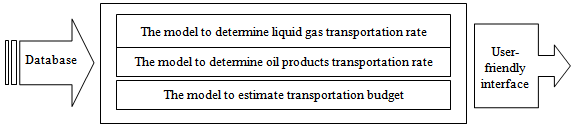 | Figure 4. System architecture |
5. Data
- • In this section, the utilized information for transportation rate calculation are explained and their sources is provided. Information that is entered to the model is:• The price of new tanker trucks and their equipments (it is calculated by linear depreciation), salvage value, and useful life.• The characteristics of used items for tanker trucks like fuel, tire, shoe, filter types and oil (it should include the unit cost, consumption level in each shipment and performance level in each month)• Different costs of tanker trucks like extending driving license credit, driver’s fees, measuring and testing operations of tanks, income tax, commission of travelling agents, third party insurance plan, health insurance plan, comprehensive insurance plan, road tax, load insurance, and loading bill.• Other information like average monthly performance (in km) in usual conditions and working days of a tanker truck in the month• Consumption variation percentage of tanker truck items and velocity reduction percentage of tanker trucks in each 36 road conditions• List of all oil sources and destinations and all features of transportation routes like route length, topography, climate conditions, road covering and traffic type.• Products characteristics like density, price, tank filling percentage, inflammable coefficient and permitted carrying volume in litres for each tanker truck• Interest and inflation rates• Information of previous year procurement (depot to depot), product consumption growth percentage in each region, depot to retailers transportation budget in different regionsThese pieces of information are collected from references like NOIPDC, Road Maintenance and Transportation Organization, Meteorological Organization, Central Bank, Central Insurance Company, Statistical Centre of the country, world wide web, Third Party Transportation Companies, Gita-Shenasi (one of local geographical organizations), and Military Transportation regulations.
6. Results
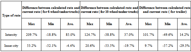
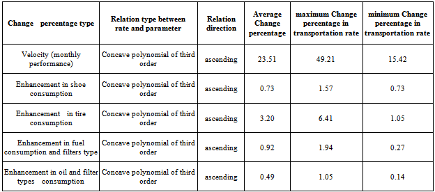
- In this section the rates calculated by the model, are compared with those which the company is currently using, and the results and comparisons are illustrated statistically Then, sensitivity analysis of the main inputs is conducted and finally, the comparison results are evaluated.In order to compare model calculated rates with the currently used ones, a number of inter-city and inner-city routes including depot to depot and depot to retailers ones are chosen as samples and then rates for these routes are calculated and results are evaluated. All rates are calculated for Kerosene (as the based product) and for each 12 months of the year. Table 7 illustrates the results statistically. Comparison between current rates (which are the same for all months and various tanker trucks) and calculated ones are depicted in minimum, average and maximum change percentages for each kind of tanker trucks.In the remainder of this section, sensitivity analysis between the calculated rate and main parameters in the model is conducted and derived results from this analysis graph are elaborated. Parameters which are involved in the sensitivity analysis are those who are probably inclined for causing error. Specifications of chosen rate for sensitivity analysis are: transportation rate for a 104 km route with totally normal conditions, for kerosene (based product), and trailer type tanker truck.An assessment of sensitivity analysis outputs shows that cost parameters like shoe, filter types and oil costs, which their value is ignorable in comparison with others, do not have a major effect on the rate. But this cannot be extended to other variables and a slight change in each of them is obviously observable in the rate. Here is parameters sensitivity analysis ranking according to their effect on the rate: monthly performance in normal situation (in Kilometres), loading and unloading time, periodic time of tire consumption, tanker trucks and its equipment purchase price and tire purchase price.As it was pointed out, for transportation rate calculation in non-baseline situation roads, considering four dimensional features of the road, some changes are applied to cash flow. These changes are considered as change percentage in the tanker truck items costs and velocity (as a result, monthly performance), and then are changed based on consumption costs period percentages and monthly performance (in Kilometers). In order to analyze the sensitivity of TRs in routes with diverse situations, a “non-asphalt, hilly, cold, normal traffic” road has been chosen and different change percentages values of monthly performance (in Kilometers) and consumption costs for that specific rate are compared. Sensitivity analysis results are illustrated in Table 8.The results of analysis show that the accuracy in change percentage of velocity or in another words traversed distance has a significant impact on making calculated rates more precise. From now on, due to considerable costs of tires, change percentage parameter of tire consumption would be paid more attention. Other items do not have a considerable impact on calculated rate. Since various situations exist in long routes, cumulative error would turn out in change percentage calculation, therefore by more accurate parameter tuning, the transportation costs for non-baseline situation can be calculated more wisely.
|
|
7. Conclusions
- Current paper introduces a systematic and scientific method for calculating the TRs for tanker trucks and at the end, explains about designing a computer-based system for calculating the TRs and estimating its required budget. In the designed technique, TRs calculation is based on the finished cost method and economic engineering techniques or time value of money method. Then, the transportation cost in a specific route and loading and unloading costs in origin and destination are estimated. The designed system is a piece of software with a user-friendly interface that based on its database which contains all the required data, calculates transportation rate for each product by each tanker truck type, in each route and month and between depot to depot and depot to retailer, and estimates the required budget for the following year.Sensitivity analysis results on problem inputs and a comparison between sample rates and currently used rates indicates that if parameter estimation is accurate enough, rates calculated by models can become a logical and scientific base for other negotiations. Regarding to the advantages that have gained from the development of this mechanism for rate calculation, constructive suggestions can be given for future researches. One can consider for a similar mechanism which targets calculating oil products transportation rate for pipelines, rail and ships. The next suggestion is to design a mechanized system to optimize Oil distribution in the country as an input for the mechanized system of rate calculation.
ACKNOWLEDGEMENTS
- This work was partially supported by NIOPDC (National Iranian Oil Products Distribution Company) under the framework of a funded research project.