Hendrik Lamsali
School of Technology Management & Logistics Universiti Utara Malaysia, 06010, Sintok, Malaysia
Correspondence to: Hendrik Lamsali , School of Technology Management & Logistics Universiti Utara Malaysia, 06010, Sintok, Malaysia.
| Email: |  |
Copyright © 2012 Scientific & Academic Publishing. All Rights Reserved.
Abstract
This research examines the reverse logistics problem in which manufacturers need to determine the collection methods for used product at the end of its life. Three collection methods are studied namely pick-up, drop-off and mail return. The research investigates the problem of assigning appropriate collection methods that can maximize manufacturer’s profit. Initially, a mixed integer non-linear programming model integrating the three collection methods is proposed to tackle the problem. In the later part, a Lagrangian heuristic approach is then proposed due to the complexity of the problem and the inability of the previous solution method to solve larger problem instances effectively. The proposed solution is tested using some problem instances and the results are promising. The issues, potential and benefits of the proposed solution are highlighted.
Keywords:
Reverse Logistics, Collection Methods, Lagrangian Relaxation, Mixed Integer Non-Linear Programming
Cite this paper: Hendrik Lamsali , An Application of Lagrangian Relaxation Approach in Reverse Logistics Problem, Management, Vol. 3 No. 1, 2013, pp. 24-30. doi: 10.5923/j.mm.20130301.06.
1. Introduction
The extended producer responsibility states that manufacturers are responsible for free taking back and recovery of their end-of-life products and must bear all or significant part of the collection and treatment costs[1],[2]. At the same time, the amount of collected returned products should at least satisfy the required minimum collection rate. It is also noted that collection of used products potentially accounts for a significant part of the total costs of any closed-loop supply chain[3],[4]. Collection effectiveness depends on the consumers’ willingness to return used products at the time of disposal[5]. It has been identified that two important factors which influence customers’ willingness to return their products are accessibility and incentives[6],[2],[7]. Customers’ convenience when returning their products should be maximized as it will eventually encourage more future returns[8]. In practice, the facilities need to be located within close proximity to the customers. Previous studies usually group customers based on geographical zones and each zone is served by one particular drop-off facility[9],[5] and[10]. In the mean time, incentives play a significant role in influencing customers’ willingness to return their products. In[9], some manufacturers were able to influence the quantity of returns by using buy back campaigns and offering financial incentives to product holders. Apart from an increment in terms of product return quantities, the amount of incentives offered by the manufacturers influences the quality level of the returned products[9]. In the mean time, there is lack of research directly addressing the aforementioned collection methods of pick-up, drop-off and mail return. Notably, studies by [9],[5] and[10] investigated problems involving one of the above collection methods (except the mail return method in which was almost non-existence). Nonetheless, each collection method was studied separately (each manufacturer used only one collection method). In practice, this situation is not helping as manufacturer faces challenges to increase collection rates as well as potential profit. Hence, this research attempts to investigate the possibility of incorporating the three collection methods together in a single model in order to maximize collection rates and potential profit. The importance of the monetary incentives and how it affects manufacturer’s profit and collection strategies when all collection methods are considered should also be investigated. The remaining parts of this article are organized as follows: problem definition is presented in Section 2 then followed by model formulation in Section 3. In Section 4, details of the application of Lagrangian relaxation method is presented. Finally, Section 5 summarizes conclusion of the research and highlight some further research directions.
2. Problem Definition
This study examines a manufacturer-typed product recovery network design. This type of collection network is practiced by many companies[11],[6]. Specific attention is given to the collection stage of product returns. At this stage, customers have several options of returning used products either via a drop-off facility, a mail delivery return or a pick up collection method provided by the manufacturer. It is up to the manufacturer to influence customers’ preference and assign them to certain collection method using the incentive offers. As long as it is technically possible and economically viable, it is assumed that customers’ decision to return their products as well as their preference over a particular collection method is heavily influenced by the amount of incentives offered. It is also assumed that customers have no other option to return their products. In this study, the manufacturer is assumed to use its forward distribution networks to collect returned products. In particular, the manufacturer may select and appoint certain retailers as collection centres/drop-off points. Customers can also be clustered into certain zones instead of being considered as individuals to reduce complexity as shown by[9]. In terms of the return flow, only one collection centre can be chosen for the customers in each zone. Hence, the function of each collection centre will not be overlapping. Meanwhile, we assume that operating costs for every collection centres are the same and all facilities are homogenous as also depicted by[9]. The vehicles used are also assumed to be homogenous. The variable cost of a pickup trip is defined by the cost per unit of distance and the distance of travelled from the collection centre to the customer zone and back. The amount of incentives offered is assumed to affect customers’ decision to return their products. The values of the incentives vary between the collection methods in order to compensate customers’ effort and their travelling costs to return their products. It is also assumed that all collected products are recoverable and hence still have remaining values to be recaptured. In terms of customers’ willingness to return their products, if the incentive offered is less than what the customers expect, then probability of customer return is zero. On the other hand, if the amount of incentive offered is equal or higher than the maximum amount of incentive that the customer expect for a particular product, then all customers will return their products. The amount of return will not change further if the amount of incentives increases above the maximum incentives that customers expect. In the mean time, the requirement by government regulations can be reflected in the form of minimum recovery rates. In this study, a manufacturer is assumed to be producing multiple products that can be returned by customers using either one of the three collection methods. Products such as ink cartridges, rechargeable batteries, disposable camera, mobile phones and books fit the bill.
3. Model Formulation
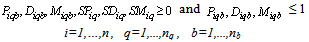
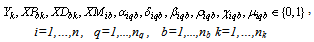
This research develops an integrated model for the manufacturer to decide the collection method for each customer zone and the amount of monetary incentives offered to customers for returning used products. The objective of the model is to find optimal assignment of collection methods to customer zones so as to maximize the total profit. The estimated amount of returned products of each type and quality classes available for return in each zone is assumed to be known. The model formulation of the drop-off collection method is based on the work of[9] and extensions have been made to incorporate other collection methods. For completeness, we introduce some parameters and decision variables that are used in the proposed model as follows:ParametersI = {1,..,n}: the set of returned product types;B = {1,..,nb} : the set of customer zones;Q= {1,..,nq}: the set of product quality classes;K= {1,..,nk}: the set of potential collection centres;TAi : Total amount of returned product type i;Tiqb: Total amount of used product type i of quality q in customer’s zone b;CDbk : Travelling cost per unit distance for drop off from customer zone b to collection centre k;Dbk : Distance between potential collection centre k and customer zone b;cv : Fixed cost of operating a vehicle; CV : Pick up vehicle’s travel cost per unit distance;Ck : Fixed cost of operating a drop-off facility k;CMi : Cost of receiving and handling a unit of product i returned via mail;CSi : Customers’ shipping/post cost to return a unit of product i via mail;KV : Maximum load (capacity) of a vehicle;KDk : Maximum capacity of a collection centre k;HPiq :Maximum incentive of product i of quality q (pick up method);HDiq :Maximum incentive of product i of quality q (drop-off method);HMiq :Maximum incentive of product i of quality q (mail delivery method);LPiq : Minimum incentive of product i of quality q (pick up method);LDiq : Minimum incentive of product i of quality q (drop-off method);LMiq : Minimum incentive of product i of quality q (mail delivery method);Riq : Expected value per unit of product i in quality class q;XRi : Required minimum collection rate for product i;W : A large number.Decision variablesSPiq : Incentive offered for product i of quality class q (pick up method);SDiq : Incentive offered for product i of quality class q (drop-off method);SMiq : Incentive offered for product i of quality class q (mail delivery method);Piqb : Proportion of product i of quality class q collected from customer zone b; Diqb : Proportion of product i of class q dropped off by customers in zone b;Miqb : Proportion of product i of quality class q returned from customer zone b ;Vbk : Number of vehicles needed to collect and transport returned products from customer zone b to collection centre k;Yk : 1, if a drop-off facility (collection centre) is setup at site k, 0, otherwise;XDbk : 1, if product owners in zone b are assigned to drop-off their products at collection centre k, 0, otherwise; : 1, if product owners in zone b are assigned for pick up collection to collection centre k, 0, otherwise;
 : 1, if product owners of product i in zone b is assigned for mail delivery method, 0, otherwise;
 : 1, If product owners in zone b do not drop off their products, 0, otherwise;
 : 1, If all product owners in zone b drop off their products, 0, otherwise;
 : 1, If product owners in zone b do not return their products (pick up), 0, otherwise;
 : 1, If all product owners in zone b return their products (pick up), 0, otherwise;
 : 1, If product owners in zone b do not return their products (mail return delivery), 0, otherwise;
 : 1, If all product owners in zone b return their products (mail return delivery, 0, otherwise.Using the above notion the problem can be formulated as the following mixed integer non-linear programming model.Max
  Where Z1, Z2 and Z3 are profits from the pickup (not counting the operating costs of collection/drop-off centres), drop-off (counting all the operating cost of the collection/drop-off centres) and mail return methods respectively.
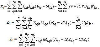 Subject to:A collection centre, k, can receive collected products from more than one customer’s zones, b, but each zone is assigned to only one collection method, and if it is assigned to pickup or drop-off method, it can only be assigned to one collection/drop-off centre as shown in (1):
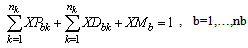 | (1) |
Returned products of all types and qualities collected via the pick-up and drop-off methods can only be delivered to a collection centre that is set up as follows: | (2) |
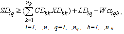
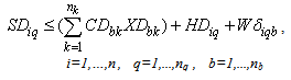
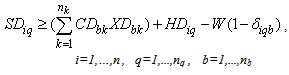
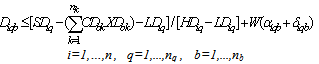
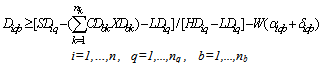
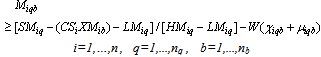
The incentive values represent customers’ willingness to return their products. In terms of the drop-off method, the relationships between the incentives and the proportion of products returned are as follows: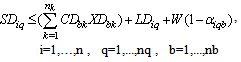 | (3) |
 | (4) |
 | (5) |
 | (6) |
 | (7) |
 | (8) |
 | (9) |
 | (10) |
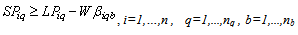
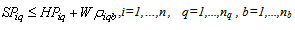
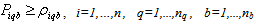
As for the pick-up collection method, the relationships are given as follows: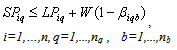 | (11) |
 | (12) |
 | (13) |
 | (14) |
 | (15) |
 | (16) |
 | (17) |
 | (18) |
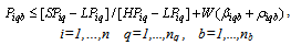
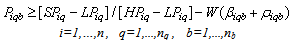
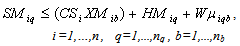
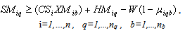
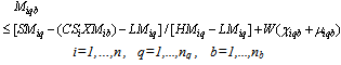
The relationships between the incentives and the proportion of products returned from zone b via mail are illustrated in the following equations: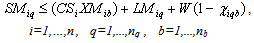 | (19) |
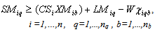 | (20) |
 | (21) |
 | (22) |
 | (23) |
 | (24) |
 | (25) |
 | (26) |
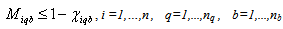
Note that constraints (9-10), (17-18) and (25-26) are active only when 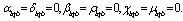 No product can be returned using a collection method if the method is not chosen as shown in (27),(28) and (29):
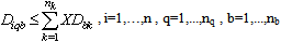 | (27) |
 | (28) |
 | (29) |
 | (30) |
 | (31) |
 | (32) |
 | (33) |
 | (34) |
 | (35) |
4. The Lagrangian Relaxation Method
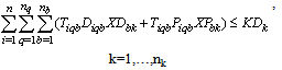
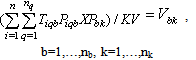
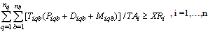
In order to relax the problem, constraints making the problem complex need to be removed and incorporated into the objective function. The selected constraints for relaxation are the capacity constraints. By dualizing the capacity constraints, the problem becomes an uncapacitated facility location-allocation problem. This situation enables each collection centre to receive as many returned products as possible without any capacity restriction. Relaxing the constraints would make the problem less complicated and more solvable. Referring back to the previous chapter, the capacity constraints are as follows: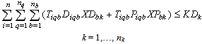 The above constraints stated that the amount of all returned products collected via drop-off and pick-up methods cannot exceeds the capacity of the opened collection centres. Let vk be the multiplier, a non-negative variable, for the constraint related to centre k. With the constraints being relaxed, the term to be added to the objective function will be as follows:
 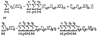 The Lagrangian relaxation problem (
 ) will beMaximize
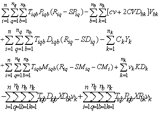 Subject to constraints (1 – 29), (31 – 34). In this case,
  is a relaxation of P1. For any non-negative values of the Lagrangian multipliers, the optimal objective value of
  provides an upper bound to the optimal objective value of P1. On the other hand, any feasible solution of P1 gives a lower bound for the objective value of the optimal solution. An iterative procedure can therefore be developed to search for the best upper and lower bounds so as to close the gap between them, through updating the value of the Lagrangian multipliers. The process of updating the multipliers should be guided by bounds so that the relaxed solution becomes closer and closer to feasible. The calculation (and updating rules) of the multiplier values is based on the general rule of (Fisher, 2004). Considering the constraints relaxed and the multipliers in this study, the multipliers are updated as follows.
 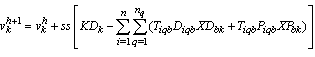 Where ss is a positive scalar step size and h is the iteration number. The calculation on the step size value is as follows:
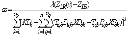 Here
Here  represents the objective value of in the current solution of the relaxed model LRp with Lagrangian multipliers v;
  represents the best lower bound up to the current iteration; and
  is a scalar satisfying
  (Held et al, 1974). The heuristic algorithm is presented in the following section.
4.1. Lagrangian Relaxation Algorithm
 produces the optimal solution to the original problem. As it is a maximization problem, the objective value of the optimal solution,
  , is the maximum objective value among all feasible solutions to the problem. Removing certain constraints such as the capacity limitation for each collection centres generates a higher objective value for the relaxed-problem (
 ). Nonetheless,
  does not necessarily guarantee feasible solutions. Some heuristic needs to be developed to generate a feasible solution based on the solution of
  . The objective value of the best feasible solution in the process will be taken as the heuristic solution of the original problem. The procedure of the Lagrangian Relaxation algorithm for the problem understudy is presented below.1. Initialize:a. Set the initial upper and lower bounds for the optimal objective value, ZUB = +
 , ZLB=
  .b. Set the maximum number of iterations, Nmax=100, and the target duality gap ε=0.001.c. Set the initial iteration number N=0, and the initial Lagrangian multipliers, vkN = 0 for all k.2. Solve the Lagrangian relaxation problem (with the capacity constraints relaxed) and denote the resulting objective value as ZLR. If ZLR < ZUB, let ZUB = ZLR.3. Test the feasibility of the Lagrangian relaxed solution for the capacity constraints. If it is not feasible, generate a feasible solution based on the relaxed solution (detailed steps will be presented in the next subsection). Denote the objective value of the feasible solution as Zfeas. If Zfeas > ZLB, let ZLB =Zfeas.4. If N >= Nmax (iteration limit reached) or (ZUB-ZLB)/|ZLB|<= ε (target gap between the best UB and LB is reached), go to Step 6.Otherwise, update the multipliers:
 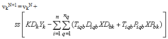 wheress = step size. 5. Let N=N+1, go to Step 2. 6. Stop. The best feasible solution found is taken as the problem solution and its objective value is
  .
.  is the best upper bound of the optimal objective value.
4.2. Steps to Generate Feasible Solutions
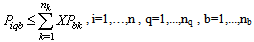
In Step 3 of the above Lagrangian relaxation algorithm, a feasible solution needs to be generated based on the solution of the relaxed problem. The following are the detailed steps for this.1. Let k=1. 2. Test the feasibility of the capacity constraint for collection/drop-off centre k: If , go to step 6; Otherwise proceed to step 3.3. For each customer zone b :if XPbk=1, let Costbk=
 ;if XDbk=1, let Costbk=
 ;if XMbk=1, let Costbk=0.4. Identify the b with the highest Costbk, denote the corresponding b as b’.5. Let XPb’k=0, XDb’k=0, XMb’k=1; go to step 2.6. If k<nk, let k=k+1, and go to step 2; Otherwise, a feasible solution has been found, the objective function value of the feasible solution can be calculated:
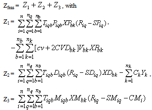
4.3. Problem Illustration and Analysis
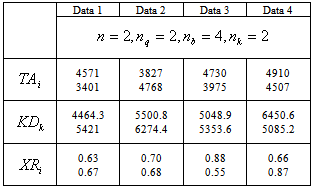
The Lagrangian Relaxation algorithm has been tested on four (4) problem instances. The experiments were conducted on a PC with Intel Core 2-powered CPU (2.13GHz) and 1.98GB RAM. The algorithm was programmed using Microsoft Visual C++, and the software package LINGO was used to solve the relaxed problems. Table 1 illustrates some of the selected parameters taken from each problem instances. Table 1. Selected parameters’ values for each of the four small sized problem instances
 |
| |
|
Where  = Total amount of returned products type i (i
 n)
n) = Capacity of collection centre k (k
  nk)
nk) = Minimum recovery rate for products type i (i
 n)As shown in Table 2, four experiments have been conducted using problem instances, each with four customer zones and two collection centers. The computational time taken to complete the whole algorithm is in seconds and recorded as CPU times. As a maximization problem, the upper bound (UB) refers to the objective function value of the relaxed solution, while the lower bound (LB) represents the best feasible solution. The relative gap between UB and LB is calculated as:
 The results depicted good performance by the proposed Lagrangian relaxation approach. In all instances, the gap is less than 3% (2.75%) while the lowest one is 0.394%. The average relative gap for these four instances is 0.9925% which is less than one percent. Of all problem instances, only one (problem instances three) produced feasible solution at the first attempt, assigning mail return delivery to all customer zones. Others generated feasible solution via the proposed feasibility approach (steps to generate feasible solution) with the solutions pointing to mixed allocation strategy between pick up and mail return or drop-off and mail return method. All solutions also satisfy the minimum recovery rates (collection rates) requirement. Based on the above table, the results show that the proposed Lagrangian Relaxation method is capable of producing a reasonable feasible solution in reasonably short computation times. The short computation time is a good potential indicator for the method’s efficiency before it will be tested using more and larger instances. The enormous saving in the computation time shows significant promises for the Lagrangian method, and it is likely more practical when dealing with larger problems. In terms of the allocation, the result in the Lagrangian Relaxation approach shows more variety or combination of collection methods.
| Table 2. Result Summary (small problem instances) |
| | Problem Instances (Data sets) | No of Customer zones (nb) | No of Collection centres (nk) | CPU Times (in seconds) | Upper bound (UB) | Lower bound (LB) | Gap (%) between UB and LB | | 1 | 4 | 2 | 293.81 | 29874 | 29073.90 | 2.75 | | 2 | 4 | 2 | 2586.86 | 193123.41 | 192323.44 | 0.416 | | 3 | 4 | 2 | 2639.51 | 203872.20 | 203072.23 | 0.394 | | 4 | 4 | 2 | 2458.48 | 198442.80 | 197642.78 | 0.41 |
|
|
5. Conclusions
This study presented analysis on product return channels (initial collection methods). A Mixed integer non-linear programming model is developed to tackle the problem. A Lagrangian relaxation approach is then proposed due to complication of the problem. The result shows promising findings indicating shorter computation times and applicability for larger problem instances. However, further rigorous examination using more problem instances is needed to further validate the findings. Important issues such as availability of the required resources and facilities needed for each manufacturer to offer all three collection methods also need further examination. In other words, there may not be many capable manufacturers out there that can offer those three collection methods simultaneously due to feasibility factors.
References
| [1] | Mansour A. and Zarei M., “A multi-period reverse logistics optimization model for end-of-life vehicles recovery based on EU Directive”, International Journal of Computer Integrated Manufacturing, vol.21, pp.764-777, 2008. |
| [2] | Shulman, JD., Coughlan, AT., and Savaskan, RC., “Optimal Reverse Channel Structure for Consumer Product Returns”, Marketing Science, Vol. 29, No. 6, pp. 1071–1085, 2010. |
| [3] | Baenas, JMHojas, De Castro, R, Battistelle, RAG, and Junior, JAG, “A study of reverse logistics flow management in vehicle battery industries in the midwest of the state of Sao Paulo”, Journal of Cleaner Production, Vol. 19, no. 2-3, pp. 168-172, 2011. |
| [4] | Dekker R, Fleischmann M., Inderfurth K., and Van Wassenhove L.N., Reverse logistics network design: Quantitative models for closed-loop supply chains, Berlin: Springer, 2004. |
| [5] | Wojanowski R., Verter V., and Boyaci T., “Retail-collection network design under deposit-refund”, Computers & Operations Research, vol.34, pp.324-345, 2007. |
| [6] | Zaarour N., Melachrinoudis E., and Min H., “Developing the reverse logistics network for product returns”, Proceeding in SPIE, vol.6385, 2006. |
| [7] | Ilgin, M.A., and Gupta, S.M., “Environmentally conscious manufacturing and product recovery (ECMPRO): A review of the state of the art”, Journal of Environmental Management, Vol.91, pp.563-591, 2010. |
| [8] | Min H., and Ko H-J., “The dynamic design of a reverse logistics network from the perspective of third-party logistics service providers”, International Journal of Production Economics, vol.113, pp.176-192, 2008. |
| [9] | Aras N, Aksen D., and Tanugur, A.G., “Locating collection centers for incentive-dependent returns under a pick up policy with capacitated vehicles”, European Journal of Operational Research, vol.191, pp.1223-1240, 2008. |
| [10] | Aras N. and Aksen D., “Locating collection centers for distance-and-incentive-dependent returns”, International Journal of Production Economics, vol.111, pp.316-333, 2008. |
| [11] | Savaskan R.C., and van Wassenhove L.N., “Reverse channel design: The case of competing retailers”, Management Science, vol.52, pp.1-14, 2006. |
 Abstract
 Reference
 Full-Text PDF
 Full-text HTML