-
Paper Information
- Next Paper
- Previous Paper
- Paper Submission
-
Journal Information
- About This Journal
- Editorial Board
- Current Issue
- Archive
- Author Guidelines
- Contact Us
Management
p-ISSN: 2162-9374 e-ISSN: 2162-8416
2012; 2(5): 149-160
doi: 10.5923/j.mm.20120205.03
Multi-objective Nurse Scheduling Models with Patient Workload and Nurse Preferences
 Abstract
 Reference
 Full-Text PDF
 Full-Text HTML
Gino J. Lim 1, Arezou Mobasher 1, Murray J. Côté 2
1Department of Industrial EngineeringThe University of HoustonHouston, TX, 77204, USA
2Department of Health Policy and Management Texas A&M Health Science Center College Station, TX 77843-1266, USA
Correspondence to: Gino J. Lim , Department of Industrial EngineeringThe University of HoustonHouston, TX, 77204, USA.
| Email: |  |
Copyright © 2012 Scientific & Academic Publishing. All Rights Reserved.
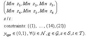
The purpose of this paper is to develop a nurse scheduling model that simultaneously addresses a set of multiple and oftentimes conflicting objectives in determining an optimal nurse schedule. The objectives we consider are minimizing nurse labor costs, minimizing patient dissatisfaction, minimizing nurse idle time, and maximizing job satisfaction. We formulate a series of multi-objective binary integer programming models for the nurse scheduling problem where both nurse shift preferences as a proxy for job satisfaction and patient workload as a proxy for patient dissatisfaction are considered in our models. A two-stage non-weighted goal programming solution method is provided to find an efficient solution that addresses the multiple objectives. Numerical results show that considering patient workload in the optimization models can make positive impacts in nurse scheduling by (1) improving nurse utilization while keeping higher nurse job satisfaction and (2) minimizing unsatisfied patient workloads.
Keywords: Nurse Scheduling, Optimization, Goal Programming, Mathematical Model
Cite this paper: Gino J. Lim , Arezou Mobasher , Murray J. Côté , "Multi-objective Nurse Scheduling Models with Patient Workload and Nurse Preferences", Management, Vol. 2 No. 5, 2012, pp. 149-160. doi: 10.5923/j.mm.20120205.03.
Article Outline
1. Introduction
1.1. Problem Description
- The cost of health care is rising every year in the United States. According to the Towers Perrin health care survey, health care costs have increased on average 6% in 2008 compared to 2007[1]. The cost of developing new technologies and treatments, America's aging population, rising personal income and generally increasing demand for health care are some of the reasons for this rapid growth in health care cost.Operations research techniques can help reduce health care costs by improving resource utilization, hospital patient flow, medical supply chain, staff scheduling, and medical decision making, to name a few. In this paper, we focus on staff scheduling, especially, nurse scheduling. Nurse shortage is a widespread problem[2]. Not having enough skilled nurses in clinical settings has caused a significant negative impact on patient outcomes, including mortality[3]. In this context, hospital administrators and nurse managers are in dire need to optimally utilize and retain currently available nurses without jeopardizing their job satisfaction. When one schedules nursing staff, it is known that considering their shift preferences can increase job satisfaction, which leads to savings in labor costs due to reduced nurse turnover and the subsequent other issues that are related with fewer nurses[4, 5].Scheduling nurses to meet a hospital's daily demand and satisfy staffing policies such as those dictated by a union contract and regulations mandating specific nurse-to-patient ratios is an extremely complex task to perform. Confounding this environment is the fact that the nurses are non-homogeneous with respect to their skill set, experience, employment type, i.e., part time versus full time, and general availability. Further, the demand for nurses varies in accordance with patient census. Because some of these objectives may conflict with each other, nurse scheduling must be carefully done to capture appropriate trade-offs among the different objectives.In this paper, we develop a nurse scheduling model that simultaneously addresses a set of multiple and oftentimes conflicting objectives in determining an optimal nurse schedule; 1) minimize nurse labor costs, 2) minimize patient dissatisfaction, 3) minimize nurse idle time, and 4) maximize job satisfaction. We formulate a series of multi-objective binary integer programming models for the nurse scheduling problem (NSP) where we use nurse shift preferences as a proxy for job satisfaction (e.g., if the nurse gets the shift s/he wants, job satisfaction is increased) and patient workload as a proxy for patient dissatisfaction (e.g., higher patient workload implies increased patient dissatisfaction). We use a two-stage, non-weighted goal programming solution method to find an efficient solution that addresses the multiple objectives. Unlike previous research[6], we define patient workload to be more than simply a care unit's census. Rather, patient workload is viewed as a factor for the care unit's case mix for a given shift. If the case mix is high, there will be a correspondingly high workload placed on nurses and, in turn, patient workload will be high. In effect, a high patient workload implies a higher workload for the nurses. Similarly, if the case mix is low, there will be low workload for the nurses. For example, if a patient requires an MRI, he may need to receive a preliminary examination, a dye injection, and the MRI procedure. Consequently, this patient requires three different services which can be considered as three separate workloads. If patient workload is less than nursing capacity, there will be idle nurses. Therefore, we define nurse idle units as the number of patient needs that could be handled by the current nursing capacity. By definition, nurse idle units will always be greater than or equal to the number of idle nurses.
1.2. Literature Review
- The research on nurse scheduling and staffing is vast and we make no attempt to review all of the literature in this domain. Rather, the literature that is relevant to our manuscript is as follows. The articles by Cheanget. al. [7]and Burke et. al.[8] might be two of the most comprehensive surveys in nurse scheduling and rostering problems. Burke et al described a general nurse scheduling and rostering problem, and evaluated various models and solution approaches found in more than 140 articles and PhD dissertations. Some of these papers can be found in[9,10,11,12]. Since then, most researchers have focused on heuristic approaches that provide an efficient solution to NSP due to the complexity of modeling and solving optimization models[13,14,15,16]. For example, Burke et. al.[17] developed a decision support system for the nurse rostering problem. They introduced a hybrid variable neighbourhood search (VNS) algorithm that can effectively handle problems with fewer than 20 nurses.Integer programming (IP) has been widely used for solving the NSP problem[13,18,19,20,21,22].Purnomo and Bard[22]introduced a new methodology using Lagrangian penalization techniques to solve an integer programming model with complex constraints to satisfy nurse shift preferences and minimizing costs considering nurses demands. Recently Belien and Demeulemeester[23] have developed an integrated nurse and surgery scheduling problem using IP and column generation methods to solve the model. A nonlinear integer programming approach was also reported in the literature[24].They highlighted how nurse-to-patient ratios and other policies impact schedule cost and schedule desirability.Most of the proposed optimization models deal with a single objective function. However, NSP is truly a multiple objective optimization problem[14,25,26,27,28]. Parr and Thompson[27] developed a multi-objective framework for a nurse scheduling problem using a weighted cost function where simulated annealing was used to solve the problem. Recently, Maenhout and Vanhoucke[25], presented a branch and price algorithm for solving a multi-objective nurse scheduling problem incorporating some penalty scores associated with scheduling inefficiencies. Other relevant nurse scheduling papers can be found in[29,30].Some papers have considered patient demand [16,31,32]. Ogulata et al[21] used an IP model to assign patients in a highly demanded hospital to physicians. They defined the patient demand and the hospital priorities without considering staff preferences.Although there is a vast amount of literature in NSP, none of the optimization models have addressed both the impact of patient workload and nurse preferences simultaneously. Therefore, our purpose here is to introduce a general and easy-to-implement multi-objective nurse scheduling problem that considers patient workloads as well as nurse preferences. Our main goal is to present the importance of adding patient workload in nurse scheduling problems.The rest of the paper is organized as follows. In Section 2, we formulate two integer programming models. The first one is the base model for nurse shift preferences and the second model includes patient workload. Both models are formulated as multi-objective optimization problems. We provide a solution algorithm for solving the models in Section 3. Numerical results are presented in Section 4 to show the effect of adding patient workload to the model. We provide concluding remarks and directions for future research in Section 5.
2. Nurse Scheduling Models
- Hospitals have their own rules and regulations for assigning nurses to shifts. Such rules and regulations can be thought of as constraints in an optimization model. Constructing a mathematical model can be quite complex if we consider all possible constraints for a given model. However, some constraints are inherently common in all hospital staffing. This leads us to develop a basic structure for a general nurse scheduling problem. One such constraints is based on shift limitations. Hospital staffing must cover 24 hours a day.Therefore, hospitals hire nurses to fulfil multiple shifts per day and these nurses fall into one of two categories of nurse types: full time and part time. Part time nurses work based on their weekly contracted work hours. Note that a hospital cannot force a nurse to work more than the regular contract hours. Therefore, nurse shortages (i.e., not having sufficient nurses to meet demand) and idled nurses (i.e., having more nurses than needed to meet demand) can add substantial labor expense to the operating costs of hospitals.Having these constraints in mind, we define two models: assignment model and patient workload model. The Assignment Model includes nurse preferences, but not patient workload while the Patient Workload Model considers both of these constraints.
2.1. Assignment Model (AM)
2.1.1. Assignment Model (AM)
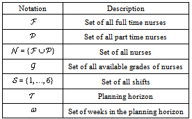
- Our aim is to assign different types and grades of nurses for hospital staffing in order to minimize operating costs. In addition to nurse types, nurses are further classified based on their skill level, work experience, certification, or other qualification criteria. The nurse scheduler decides how many shifts the hospital needs per day. We define a shift as a consecutive 4-hour period such that we have 6 shifts per day. Sometimes, due to nurse shortages, higher skilled nurses can be assigned to shifts that lower skilled nurses are often assigned to. However, the opposite is not appropriate because it equates to poor quality of care or an inappropriate or illegal use of resources. A master schedule can be developed for each scheduling period such as a week, month, or quarter. Based on this information, we define the following indexes in Table 1.
|
2.1.2. Input Parameters
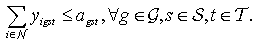
- There are several input parameters to the optimization model. First, the nurse schedule will be constrained by the number of available nurses (
 ) that a hospital has for a specific shift. If there is a need for more nurses than this number (
 ), the hospital will experience a shortage of nurses for the shift. As stated before, this shortage of nurses can add to the hospitals operating cost. By the same token, any idle nurses will contribute to this cost because the hospital is not fully utilizing its workforce. We define
  as the number of available nurses for each grade
 ,shift
 and day
  .Second, hospitals assign different nurses to different tasks based on their skill level (grade). Assuming that nurse grades are given as input, we define nurse grades in the model as follows:
 = 1, If the grade of nurse
  is higher or equal
  ; 0, otherwise.Since each type of nurse has a different compensation structure per shift per day, the third input is the cost of assigning a nurse to a shift;
  . The next input is the type of contract such as full time and part time. We assume that each nurse works up to their contracted hours, i.e., we do not consider overtime. We address this issue by hiring part time nurses so that overtime is not necessary in the model. All nurses can be assigned to shifts that include days, nights, and weekends. Other additional input parameters are defined as follows:
 : Number of shifts nurse
  mustwork in a week,
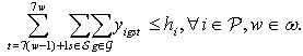
 : Maximumnumberoflate nightshifts a fulltime nursecanbeassigned to, in the planning horizon,
 : Maximum number of weekend shifts a fulltime nurse can be assigned to, in the planning horizon,
 : Minimum number of nurses assigned to each shift,
 : Penalty score of assigning a nurse
  to a shift
  based on nurses preference,
 : Penalty of utilizing part time nurse
  in the scheduling,
 : Penalty of assigning higher grade nurses to late night and weekend shifts,
 : Penalty of assigning fulltime nurses to late night and weekend shifts.
2.1.3. Decision Variables
- Our task is to determine which nurse should be assigned to which shift of each day. Therefore, the decision variables of the optimization model are defined as follows:
 , if nurse
  with grade
  is assigned to shift
  in day
 ; 0, otherwise.
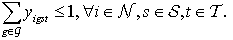
2.1.4. Constraints
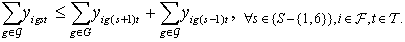
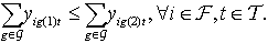
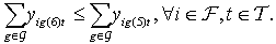
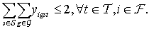
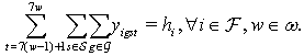
- Nurse Grades: Each nurse has a grade that reflects the skill sets one has. This grade will determine what kind of tasks the nurse has the authority and capability to perform. Typically, a nurse with a higher grade can perform tasks that a nurse with a lower grade performs. Equation (1) writes this constraint:
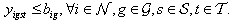 | (1) |
 | (2) |
 | (3) |
 | (4) |
 | (5) |
 | (6) |
 | (7) |
 | (8) |
 | (9) |
 | (10) |
 | (11) |
 | (12) |
 | (13) |
 .
. | (14) |
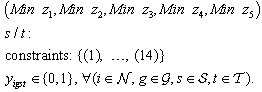
2.1.5.Objective Functions
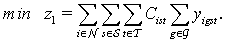
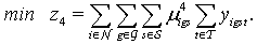
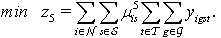
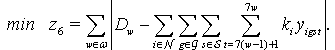
- There can be many goals in scheduling nurses such as minimizing the nurse assignment cost, maximizing nurse job satisfaction, or any other goals that the hospital has set in terms of scheduling nurses. Some of these goals may naturally conflict with each other. In this subsection, we categorize two groups of objectives. One of these groups is common to perhaps all hospitals, i.e., minimizing assignment cost and maximizing nursing job satisfaction, while the second group addresses specific hospital requirements or conditions.Minimizing Assignment Cost: Cost of assigning nurses to each shift is one of hospital's main concerns. Therefore, we define our first objective function to minimize nurse assignment cost. The total cost will be based on the hospital's compensation structure that includes salary, benefits, and any other extra expenses that the hospital must be responsible for hiring nurses:
 | (15) |
 | (16) |
 | (17) |
 | (18) |
 | (19) |
 | (20) |
2.2. Patient Workload Model (PWM)
- We extend our assignment model to incorporate patient workload in the optimization model. This model is intended to show how patient workload can affect the outcome of the model, (i.e., nurse scheduling). It is basically the assignment model with an extra objective function and auxiliary constraints.For the workload model formulation, we need to know how many patient workloads a nurse can handle in each day (
 ); namely, a nurse-to-patient ratio. Based on
  , we can determine the number of patient workloads that a nurse should be assigned to per shift. We define satisfied customers as the total number of patient workloads who receive hospital care during the scheduling period. In addition, we need to know the estimated patient workload based upon the hospitals census (
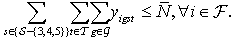
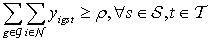
 ) over the planning horizon.Patient Workload Requirement Constraint: We may not be able to meet all demands that patients request. However, our goal is to provide the hospital care to at least β percentage of the total patient workload to increase customer satisfaction.
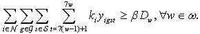 | (21) |
 | (22) |
 | (23) |
3. Solution Method
- The optimization models that we attempt to solve have multiple objectives. Many algorithms have been reported for solving multi-objective optimization (or goal programming) models (MOOM)[37]. Two main categories of solution approaches are the Weight method and the Preemptive method[38]. Both of these methods require that the decision makers prioritize the objective functions. The most common solution approach is the weighted sum method. In this approach, a new objective function is developed based on a linear combination of the goals:
 | (24) |
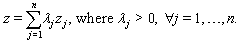
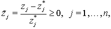
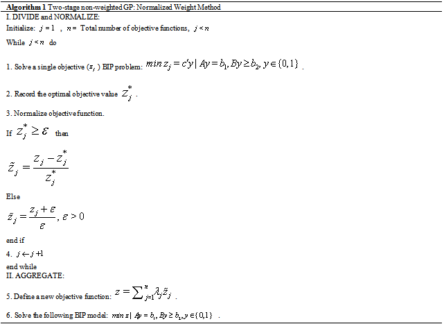 Decision makers will first rank the goals (i.e., objective functions) based on their perceived importance of each goal against other ones. Then weights will be assigned to the objective functions in such a way that the relative importance will be accounted appropriately. The process of selecting weights (λ) can be a daunting task. Many approaches have been developed for addressing this problem[39]. We note that a weighted objective function with carefully selected weights sometimes may not guarantee that the final solution will be acceptable. In this case, the decision maker needs to redesign the weights based on the outcome of the previous trial. The second issue is that the objective functions often have different scales in magnitude. This difference in scale makes it more difficult to select appropriate weights. We address these issues by applying the Normalized Weight Method as shown in Algorithm 3. This method provides a non-dimensional objective function to make weight selection easier. Our method is comprised of two stages: 1) Divide and Normalize and 2) Aggregate. In stage 1, single objective optimization problems with a set of constraints in Section 2.1.4 are solved one at a time:
 | (25) |
 , and then dividing,
  , by the optimal objective value
  .Note that
  may take a value of zero. This will cause the specific division not to be defined. We fix this problem by adding a small value ε to both the numerator and the denominator[40]. In stage 2, the multi-objective function is regrouped by a linear combination of the normalized functions and solves the following optimization problem to find an optimal schedule:
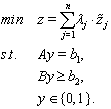 | (26) |
 in the optimal solution of (26).Observation 2: In the BIP model (26), the objective function
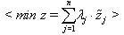 | (27) |
 | (28) |
 in our optimization models.We do not claim that our method will resolve all the inherent issues that the weighted sum method has, such as finding appropriate weights that reflect the relative importance of each goal, producing solutions that are not Pareto efficient. But, we attempt to ease the process of ranking (or rating) different objectives by normalizing the scale of the objective function values, and then assign the weights if it is necessary. Numerical results are presented in Section 4 to show the effect of adding patient workload to the model.
|
|
4. Numerical Results
- In Section 2, we have discussed two multi-objective optimization models. The assignment model is a typical nurse scheduling model that does not consider patient workload. Since one of our aims is to understand the effect of considering patient workload in the model, we have proposed the patient workload model. In Section 3, we have provided an improved method for solving multi-objective optimization problems. Therefore, numerical experiments are designed in this section to analyze the behavior of these models with and without patient workload, and to test computational performance of our proposed solution algorithm.First, we define the shifts over consecutive four hour interval starting at midnight. This means that there are six shifts per day: (midnight to 4 a.m.), (4 a.m. to 8 a.m.), …, and (8 p.m. to midnight). Based on this assumption, we generated two data sets to test our models and to show the efficiency of the solution algorithm in two different nursing capacity configurations. The first set of data (Section 4.1) contains 10 full time and 6 part time nurses while the second set of data (Section 4.2) consists of 20 full time and 6 part time nurses. In order to understand the behavior of our model, multiple patient workload scenarios are generated. For each scenario a set of 10 experiments have been implemented and the solution time is calculated based on the average solution time of all the experiments. Optimization models are formulated in GAMS and solved using CPLEX 12.1 on a Workstation with 2.8 GHz Intel Xeon quad CPU running Windows Server 2008 R1 with 16GB RAM.
4.1. Test Data Set I
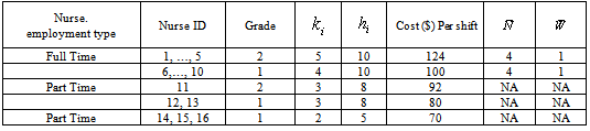
- Consider a care unit that can have at most 10 full time and 6 part time nurses (see Table 2). The full time and three part time nurses have two different grades while the other three part time nurses have only one grade. Their weekly working hours and the compensation per shift is given in the table. Other input data includes the number of weekly patient workload, the number of patient workloads that each nurse can handle,
 , the number of weekly shifts that each nurse must take,
  , the maximum number of weekly allowable late night shifts,
  , and the weekend shifts,
  .First, we calculate the hospitals nursing capacity (i.e., the maximum amount of patient workload that the hospital can handle) in our case study. We then calculate the total number of patients that a nurse
  can handle per week,
  :
: As a result, the current nursing capacity is a workload of 552
  . If the workload exceeds 552, we will experience patient dissatisfaction. Otherwise, there will be idle nurses, which are considered a non-productive resource in the hospital operation. Therefore, our optimization models attempt to minimize either the idle nurses or patient dissatisfaction.
4.1.1. Results on the Assignment Model
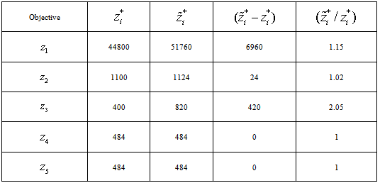
- Assignment model (20) has five objectives. The solution output of this model is summarized in Table 3. The second column
 contains the optimal objective values of the single objective optimization models described in Section 3. The third column contains objective values of all five objective functions when the multi-objective optimization model (20) is solved using the solution method described in Section 3. It is easy to verify that
 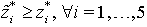 . The optimal value of the final objective
  (See equation (28) with
  ) is approximately 6.23. The model was solved in 2.78 seconds. If all the objective functions could reach their respective optimum solution, then
  would have been 5. But the multi-objective nature of this problem forces some objectives to reach sub-optimality. In our example, the solution has met nurse preferences (
 and
and  ) while we may need to hire more part time nurses (
 ). Of course, if there is a need to decrease the number of part time nurses, we would assign a higher value of
  in the optimization model to achieve this goal.
4.1.2. Results on the Patient Workload Model
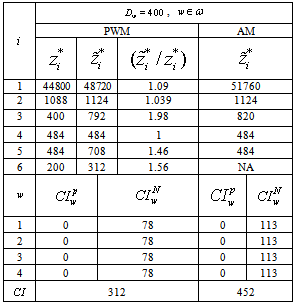
- We continue our experiments with the patient workload model described in Section 2.2. The objective function consists of six objectives. The patient workload model is solved using Algorithm 1 with
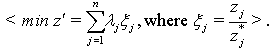
 for two cases; one with a total of 400 patient workloads and the other with 552 patient workloads. The model was solved in 3.16 seconds for the case with 400 patient workloads and in 3.74 seconds for the second case. The results are shown in Table 4. In order to compare two different models, we have added a comparison measure formula
  using equation (29) in each table and it is defined as
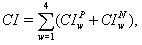 | (29) |
 is the amount of workload unsatisfied in week
  due to the lack of nursing staff and it is expressed as
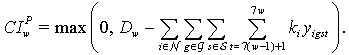 | (30) |
 is the total nurse idle units per week due to too many nurses and the lack of patient workloads to fully utilize the nursing staff and it is expressed as:
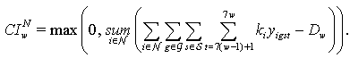 | (31) |
 and
and  ) can be useful when the scheduler wants to know if more nurses are needed or idle nurses can be assigned to different care units in the hospital.Tables 4a and 4b show a comparison between the patient workload model and the assignment model on five objectives. In the case with 400 weekly patient workloads, the fourth goal (i.e., to assign higher grade nurses to regular day shifts,
  ) reached its optimum value while
  and
and  attained near optimal solutions. The normalized objective value of the third objective function (i.e.,
  ) is close to 2, which is far from 1 (the optimal). We reason that this finding is because the pay rates of the part time nurses are much lower than the full time nurses in this particular case study.Note that the workload model has a
  value of 312 which is smaller than 452 of the assignment model. Since there is a smaller workload than the nursing capacity of 552, both models show zero values of
  . On the other hand, AM shows higher values of
  than PWM because AM does not include
  in the objective function. This indicates that adding the patient workload goal to the problem improves the nursing staff utilization.
|
|
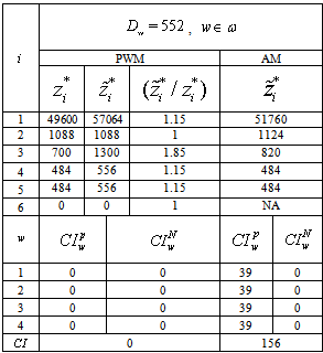
 values are zero for both of the models. This has all workload satisfied for PWM but a deficit of 39 for AM.We make the following two observations based on these results. First, PWM has a lower number of unsatisfied workloads and a lower number of nurse idle units. We speculate that this happens because PWM considers minimizing patient workloads as well as minimizing nurse idle units in the objective function. Second, in order to satisfy workloads, PWM favors hiring more part time nurses. As a result, PWM has a higher value of
  than AM.
4.2. Test Data Set II
- We now consider a care unit that can have at most 20 full time and 6 part time nurses. The full time and three part time nurses have two different grades while the other three part time nurses have only one grade. We generated this data based on Table 2 and have doubled the full time nurses. Therefore, our nursing capacity is 1002
 total number of patient workloads.
4.2.1. Results on the Assignment Model
- The solution output of this model is summarized in Table 7 in Appendix. The optimal value of the final objective (
 ) is 5.43 and the model was solved in 59.67 seconds. The results show that the behavior of the model is similar for both data sets. It is easy to see that we do not need to hire many part time nurses because we have more full time nurses. Hence, value of
  in data set II is smaller than that of data set I. Overall, increasing the number of full time nurses did not affect much on nurse preferences.
4.2.2. Results on the Patient Workload Model
- Two scenarios are run for the patient workload model; one with 800 total patient workloads and the other with 1002. The model was solved in 60.38 seconds for the first case and in 65.48 seconds for the second case. The results are shown in Table 8 in Appendix. The results from the second data set show a similar performance compared to the first data set. One thing to note is that data set II had a smaller value of
 , which means that it is easier to satisfy patient workloads since we have more available nurses. In both cases,
  values of PWM are lower than those of AM. This indicates that adding the patient workload goal to the problem indeed improves nursing staff utilization in both data sets.
4.3. Sensitivity Analysis
- We have shown that adding patient workload to optimization models can make positive impact in nurse scheduling in the previous section. We now analyze the behavior of our models under different patient workload scenarios and make performance comparison between the models. An ideal nurse schedule should satisfy both the nurses and the patients. In reality, they are often conflicting goals. So the question is which model performs better in both of these measures? We perform a sensitivity analysis of these models on patient workloads to answer this question.
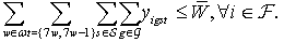
4.4. Customer Satisfaction
- Customer satisfaction can be considered for both the nurses and the patients in the hospital. Nursing staff job satisfaction can be accommodated by trying to schedule them according to their preferences. From the hospital point of view, the scheduler wishes to utilize its nurses at its optimal level, i.e.
 . Therefore, if the workload is well below its nursing capacity, the hospital has an opportunity to improve its operating cost by reducing part time nurses or re-assigning certain nurses to different care units that experience high volume of patient workloads. On the other hand, the scheduler may also wish to satisfy as many of the anticipated workloads as possible so as to minimize patient dissatisfaction.Nurse shortage is a concern that many hospitals are facing nowadays. In many cases, hospitals may not be able to satisfy its weekly patient workloads. Therefore, our workload model has constraint (21) that sets an upper bound on what percent of patient workloads must be satisfied. One can change the value of β based on the nursing capacity. Furthermore, this model can be useful in estimating how much workload will not be satisfied given that the nursing capacity is fixed. Based on this, we conducted a sensitivity analysis using different values of β and the results are displayed in Table 9 in Appendix. We calculate the amount of unsatisfied workloads (
 ) and nurse idle units (
 ) for workloads ranging from 300 to 650 for the assignment model and the patient workload model with
 ,
,  ,
,  and
and  for test data set I.Figure 1 shows the comparison between AM and PWM for
  . Figure 1 shows the comparison on
  , where the horizontal axis represents patient workload and the vertical axis is for nurse idle units. In Figure 1, the vertical axis represents unsatisfied patient workloads (
 ). For both
  and
and  , PWM performs better than AM by providing fewer
  s when the workload is less than 525 and fewer
  s when the workload is higher than 500. Evidently, increasing workload will lead to a smaller nurse idle units and more unsatisfied workloads. But, it is clear that the workload model has smaller nurse idle units as well as smaller unsatisfied workloads than the assignment model in all cases tested.Table 5 shows a nursing schedule comparison between the assignment model and the workload model for test data set I. This table shows how many full time nurses (
 ), part time nurses of type 1 (
 ), and part time nurses of type 2 (
 ) are scheduled to work based on different patient workload levels. Since there are 10
  s, 3
s, 3  s, and 3
  s, we add three columns for
  s (namely,
  ,
,  and
and  ) and another three columns for
  s (namely,
  ,
,  and
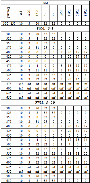
and  ) that indicate how many hours each part time nurse is assigned to work. A cell with “inf” indicates that the solution is infeasible for the specific parameter setting. As we can see from the table, the assignment model solution remains the same for all levels of patient workload. It is because AM does not consider patient workload. Due to the same reason, the AM schedule assigns all full time nurses and part time nurses of type 1 for all workload levels. This is clearly not the case when we consider patient workload in the model. In PWM, different types of nurses are scheduled to work with different hours in order to reduce
  s while meeting the patient workload. For example, when the workload is 500 and
  , in addition to 10 full time nurses, 2
  s are hired to work 21 hours and 11 hours and all three
  s are hired to work 17, 17, and 18 hours, respectively. If we decrease the value of
  to 0.9, the schedule includes 2
  s with 32 hours and 1
  with 4 hours. We notice that some part time nurses work less than 32 or 20 hours. This is an example of a rotating nurse who works for several different divisions in the hospital.
|
 ), PWM can find a feasible solution when the workload level is less than 552. As the level of customer satisfaction requirement decreases (
 ), the workload model finds feasible solutions for workloads up to 600, which is about 10% more than the current nursing capacity. In reality, this strict constraint can be easily removed to find a feasible solution, which is a compromise between patient dissatisfaction and the limited nursing capacity.
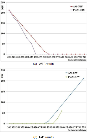 | Figure 1. Comparison between AM and PWM with  : (a) : (a)  results; (b) results; (b)  results results |
4.4.1. Nursing Staff Satisfaction
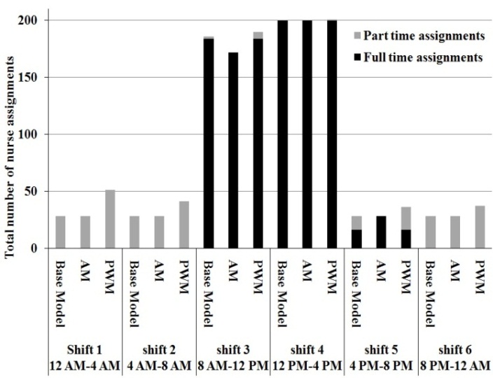 | Figure 2. Total daily shift assignment comparison of the three optimization models with  , ,  , ,  |
 ) | constraints (1),…, (14) , and (21)}.
|
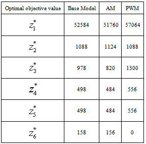
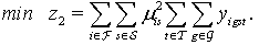
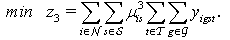
 .The results are shown in Figure 2 and Table 6. Figure 2 depicts the performance comparison for the total daily shift assignments among three optimization models. The horizontal axis represents the shift number and the vertical axis shows frequency of each shift assignment based on a four week schedule. The bars have two patterns. The darker (bottom) part is the count for full time nurses and the gray (upper) portion is for the part time nurses.Evidently, shifts 3 and 4 are most preferred in our test data set. Thus, assigning more full time nurses to shifts 3 and 4 will be ideal. This is clearly the case for the base model that considers only the nurse preference. In shift 3, AM has a lower frequency than the base model because AM has multiple objectives to compromise. Table 6 shows this trade-off. The base model has the smallest value of, which is the smallest deviation from the nurse preference. But the rest of objective values of the base model are higher than those of AM. This confirms that meeting nursing staff preference only can come at the cost of unsatisfied patient workloads. That is one of the main reasons why PWM has higher frequency for all shifts in Figure 2. Securing more (especially part time) nurses will not only make it easier to process more patient workloads, but also helps reduce the idle nurse units. As a result, PWM generates a schedule with smaller
  and
and  .
.5. Conclusions
- We have developed a series of two multi-objective nurse scheduling models: the assignment model considered labor costs and nurse preferences while the patient workload model added patient workload information to the optimization model.Because solving the assignment model is computationally expensive, a two-stage non-weighted goal programming solution method was developed to find an efficient solution quickly for these models. In order to understand the effects of adding patient workloads in the model, we introduced a comparison index that captured unsatisfied patient workloads and the idle nurse units. Based on the representative case studies, it is clear that adding patient workload into the optimization model can not only improve patient satisfaction by decreasing the unsatisfied patient workloads, but also can improve nurse staff utilization by minimizing nurse idle units. These goals can be achieved without creating higher levels of nursing staff dissatisfaction. We also showed that our solution algorithm can find optimal solutions in a reasonable time: it took about 1 minute to find a schedule for a hospital with 20 full time and 6 part time nurses.Naturally, having patient workload information can help estimate an optimal nursing staff capacity. When there is a seasonal workload pattern (e.g., flu seasons), schedulers can easily apply a forecasting approach to estimate the workload. Then our optimization models can be modified to produce how many nurses they need to acquire in order to maximize staff utilization for the scheduling period. Our future work will consider such nurse and patient workload uncertainty.