P. A. Owusu1, 2, L. DeHua2, E. K. Nyantakyi1, 3, R. D. Nagre2, 4, J. K. Borkloe1, 3, I. K. Frimpong4, 5
1Department of Civil Engineering, Kumasi Polytechnic, Kumasi, 00233, Ghana
2College of Petroleum Engineering, Yangtze University, Wuhan, 430100, China
3College of Geosciences, Yangtze University, Wuhan, 430100, China
4Department of Chemical Engineering, Kumasi Polytechnic, Kumasi, 00233, Ghana
5College of Geophysics, Yangtze University, Wuhan, 430100, China
Correspondence to: P. A. Owusu, Department of Civil Engineering, Kumasi Polytechnic, Kumasi, 00233, Ghana.
| Email: |  |
Copyright © 2012 Scientific & Academic Publishing. All Rights Reserved.
Abstract
Saturated gas drive reservoirs are characterized by rapid and continuous decline of reservoir pressure. The resultant effect of this phenomenon is the early decline of reservoir performance at the primary stage of the life of the reservoir. The recovery of hydrocarbon from this type of reservoir through the conventional lifting (spontaneous production) is inefficient and uneconomic due to its least recovery efficiency leading to significant amount of residual oil. The Muskats model was used to analyze solution-gas drive reservoir and predict its primary oil recovery. The inflow performance of the reservoir was analyzed through the Fetkovich model. Outflow performance of various tubing sizes such as 2”, 2.5”, 3” and 4” was analyzed. The future performance of reservoir is forecasted in the three stages: the first one is to predict cumulative hydrocarbon production as a function of declining reservoir pressure, the second stage is time-production phase, and the third stage of prediction is the time-pressure phase. From the inflow performance relationship IPR analysis the maximum inflow rate obtainable is 1710bpd with outflow rate of 1200bdp. The flow capacity near the abandonment reaches 77bpd at about 15925days with cumulative oil produced as 7M Mstb.
Keywords:
Solution Gas Drive, Recovery, Inflow Performance, Outflow Performance, Tubing String
Cite this paper: P. A. Owusu, L. DeHua, E. K. Nyantakyi, R. D. Nagre, J. K. Borkloe, I. K. Frimpong, Prognosticating the Production Performance of Saturated Gas Drive Reservoir: A Theoretical Perspective, International Journal of Mining Engineering and Mineral Processing , Vol. 2 No. 2, 2013, pp. 24-33. doi: 10.5923/j.mining.20130202.02.
1. Introduction
Saturated gas drive is one of the depletion drive reservoirs in which the principal drive mechanism is the expansion of the oil and its originally dissolved gas as well as the associated pore space. The increase in fluid volumes during the process is equivalent to the production. As pressure is reduced rapidly and continuously in this type of reservoir remarked by[1], oil expands due to compressibility and eventually gas comes out of solution from the oil as the bubble point pressure of the fluid is reached. The expanding gas provides the force to drive the oil hence the term solution gas drive. It is sometimes called dissolved gas drive[2]. In solution gas drive reservoirs the initial condition is where the reservoir is under-saturated, i.e. above the bubble point. Production of fluids down to the bubble point is as a result of effective compressibility of the system. This part of the depletion drive may be termed compressibility drive. The low compressibility causes rapid pressure decline in this period and resulting low recovery. Below the bubble point, the expansion of the connate water and the rock compressibility are negligible hence as the oil phase contracts owing to the release of gas from solution, oil production therefore occurs as a result of expansion of the gas phase.When the gas saturation reaches the critical value, the free gas begins to flow. At fairly low gas saturations, the gas mobility, kg/ug, becomes large and the oil mobility, ko/uo, is small, resulting in high gas-oil ratios and in low oil recoveries, usually in the range of 5 to 25%[3]. The under recovery of this type of reservoirs make them the favorite for secondary recovery applications[4]. The behavior of the saturated gas drive makes the prediction of it recovery a complex one due to continuous changing of the gas and oil viscosities as well as the volume formation factors as a result of the pressure drops. Due to the inherent complexities, a number of simplifying assumptions are advanced to develop simple mathematical models. Several methods including Muskat’s method, Schilthius’ method, Tracy’s method and Tarner’s method have appeared in literature for predicting the recovery performance of this type of reservoirs based on rock and fluid properties The Muskat’s method gains a slight advantage over the others as seen in its wide application due to its simplicity. Furtherance to this, the analysis of the reservoir deliverability as to estimate the production rate at any given flowing bottom-hole pressure is a key to forecasting reservoir performance[5]. [6] has proposed an empirical inflow performance relationship (IPR) that has been used in the industry successfully. The IPR combined with the vertical tubing (outflow) performance serves as approach to well performance analysis. The objective of this research was to investigate into the effects of tubing size on flow capacity, how cumulative production relates to the decline pressure and time and how average reservoir pressure declines with time.
1.1. Saturated-Gas Drive Reservoirs
This driving form may also be referred to as solution gas drive, dissolved gas drive, internal gas drive and depletion drive mechanisms. In this type of reservoir the principal source of energy is a result of gas liberated from the crude oil and subsequent expansion of the solution gas as the reservoir pressure is reduced below the bubble point pressure. As pressure falls below the bubble point pressure, gas bubbles are liberated within the microscopic spaces[2]. The bubbles expand and force crude oil out of the pore space.[3] suggested that the saturated gas drive can be identified by pressure behavior, water production and unique oil recovery. The reservoir pressure declines rapidly and continuously in saturated gas drives. The decline in the pressure is attributed to the fact that no extraneous fluids or gas cap are available to provide a replacement of the gas and oil withdrawals. There is little or no water production with the oil during the entire producing life of the reservoir. The reservoir is also characterized by rapidly increasing gas-oil ratio from all well, regardless of their structural position. After the pressure has reduced below the bubble point pressure, gas evolves from solution throughout the reservoir. Once the gas saturation exceeds the critical gas saturation, free gas begins to flow toward the wellbore and the gas-oil ratio increases. The gas will also begin a vertical movement due to gravitational forces, which may result in the formation of a secondary gas cap. Oil production is the least efficient recovery method in this drive. The performance of this reservoir is largely described by the gas oil ratio (GOR) as shown in (Fig. 1). In that the GOR tends to remain constant at initial gas solubility (Rsi) until pressure reaches the bubble point. GOR declines below the bubble point as gas begins to evolve from solution and its saturation increases and begins to flow as gas saturation reaches critical value. Beyond this point the GOR increases rapidly and continuously up to the maximum and then declines to mark the end of the field as pressure depletes completely[4].
1.2. Principal Recovery Models in Dissolved-Gas Drive Reservoirs
Literature is replete with several methods of forecasting the performance of the dissolved-gas drive reservoirs where deterioration of pressure is regarded as a function of GOR, oil recovery, and produced oil. These methods include Muskat’s method, Schilthius’ method, Tracy’s method and Tarner’s Method. Due to the complexity of this type of reservoirs a number of simplified conventions are made to make their solution reasonably simple[3]. Among them includes the fact that the reservoir is uniform at all times regarding porosity, fluid saturations and relative permeabilities. It is also assumed that uniform pressure exit throughout in both gas and oil zones which implies that gas and oil volume factors, gas and oil viscosities as well as solution gas will remain the same throughout the reservoir. It is further assumed that there is equilibrium at all times between gas and oil phases with negligible gravity segregation forces and negligible water encroachment and production.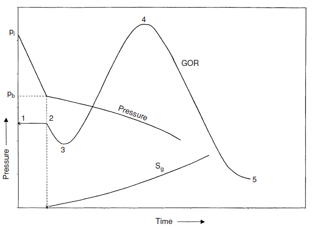 | Figure 1. Ideal Production behaviour of a saturated gas-drive reservoir |
2. Materials and Methods
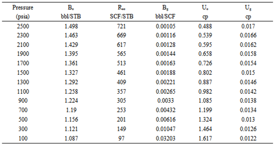
Volumetric depletion drive reservoir that exists at its bubble point pressure of 2500 psi with relevant reservoir data provided in Table 1. (Fig. 2) shows the reservoir’s total liquid saturation and relative permeability. Also, detailed fluid property data are provided in Appendix 1. Other relevant information includes: Initial Reservoir Pressure (pi = pb) = 2500 psi, Initial Reservoir Temperature = 180oF, Initial Oil in Place (N) = 56 MMSTB, Initial Water Saturation (Swi) = 0.2 and Initial Oil Saturation (Soi) = 0.8.| Table 1. Available Oil Well Data |
| | Average reservoir pressure | = 2500 psi | | Water cut | = 0% | | Initial gas – Liquid ratio (GLRi) | = 721 scf/stb | | Productivity index, J* | = 1.5 | | Gravity | = 25o API | | Specific gravity to gas | = 0.7 | | Average temperature | = 180oF | | Wellhead pressure | = 150 psi | | horizontal | = 90o | | Reservoir depth | = 7500 ft |
|
|
 | Figure 2. Permeability ratio relationship |
2.1. Application of Muskat's Method in Predicting Oil Recovery
Muskat’s method was employed in the prediction due to its wide application, simplicity and the size of the available data. In the Muskat’s method, the values of the many variables that affect the production of gas and oil and the values of the rate of changes of these variables with pressure are evaluated at any stage of depletion pressure. Assuming these values hold for small drop of pressure, the incremental gas and oil production can be evaluated for these small pressure drops. Muskat expressed the material balance equation for a dissolved drive reservoir in a simplified form as 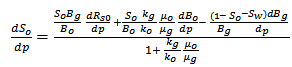 | (1) |
The above equation is simplified further on the account of the pressure functions; as X(p), Y(p) and Z(p).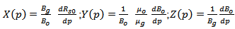 | (2) |
Equation 1 takes the form 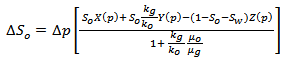 | (3) |
Equation 3 accounts for a change in oil saturation with respect to an incremental drop in pressure. The pressure functions are derived from the reservoir fluid properties. The values of  , and
, and  are derived graphically. Better results are obtained, if values at the middle of the pressure drop interval are used. This is done by simply finding the product of
  and the pressure drop
  , then subtracting the value of
  from the oil saturation that corresponds to
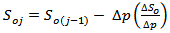 | (4) |
2.2. Instantaneous Gas-Oil Ratio (GOR)
The Produced gas-oil ratio (GOR) at any particular time is the ratio of standard cubic feet of total gas being produced at any time to the stock-tank barrels of oil being produced at that same time. GOR which is given by equation 5 predicts the reservoir performance at any time in the life of the reservoir.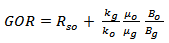 | (5) |
There are three types of gas-oil ratios; instantaneous gas oil ratio (GOR), solution gas oil ratio (Rs), and cumulative gas oil ratio (Rp). The solution gas oil ratio is given by equation 6. | (6) |
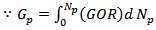 | (7) |
The incremental cumulative gas produced,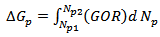 | (8) |
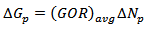 | (9) |
Between  and
and  , the above equation can be approximated to:
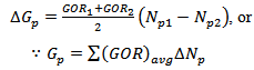 | (10) |
2.3. The Reservoir Fluids Saturation Equations
The solution of reservoir fluids (oil, gas, and water) in the reservoir at any time is defined as the ratio of volume of the fluid to the pore volume of the reservoir. and
and  , then
 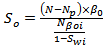 | (11) |
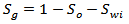 | (12) |
The reservoir PVT data must be available in order to predict the primary recovery performance of a depletion-drive reservoir in terms of Np and Gp. These data are initial oil-in-place (N), hydrocarbon PVT, initial fluid saturations, and relative permeability data. All the techniques that are used to predict the future performance of a reservoir are based on combining the appropriate MBE, with the instantaneous GOR using a proper saturation equation. The procedure is a repetitive one at series of assumed reservoir pressure drops.
2.4. Inflow Performance Relationship (IPR)
The IPR describes the two phase flow in the porous medium by appropriate models such as Vogel, Fetkovich, Standing, and Wiggins’s, The IPR is established by plotting the gross flow rate at different values of the bottom hole flowing pressure. All IPR curves are parallel to each other. The well potential decreases with the decrease in the reservoir pressure and as the pressure inside the reservoir goes below the bubble point gas evolve out of the solution reducing the viscosity of oil[2]. This has the effect of making the formation volume factor greater than one. The combined effect of this is the reduction in the productivity of oil due to the energy which is spent much on moving the liquid and gas phase[7]. The constant productivity index (PI) concept is no longer valid as the pressure is below the bubble point. The fetkovich empirical correlation was used to estimate the IPR of the reservoir. In the saturated region where p < pb, Fetkovich shows that the (PI) changes linearly with pressure as seen in (Fig. 3).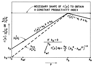 | Figure 3. Schematic mobility-pressure behaviors for solution-gas drive reservoirs[Fetkovich, 1973] |
2.5. Fetkovich’s Correlation
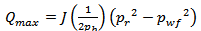
In 1968 Vogel[8] established an empirical relationship for flowrate prediction of solution gas drive reservoirs in terms of the wellbore pressure based on reservoir simulation results. Later[6] proposed a “pressure squared” deliverability relation using pseudo-state theory. When the reservoir pressure pr and bottom-hole flowing pressure pwf are both below the bubble-point pressure pb, the pressure function f(p) is represented by the straight-line relationship as expressed by Equation 13.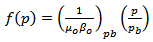 | (13) |
Equation 13 is expanded to account for the flowrate as pressure declines in field units as shown in equation 14.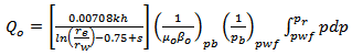 | (14) |
Integrating equation 14 gives 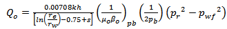 | (15) |
 | (16) |
Where the productivity index 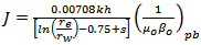 Equation 16 gives the maximum flow rate or the absolute open flow (AOF).Fetkovich’s correlation for the reservoir IPR is much simpler yet theoretically consistent alternative to Vogel IPR formulation. For detail formulations of Vogel see[8]. Fetkovich correlation was considered as it gives better practical applications[9]. Fetkovich deliverability relation is given by equation 17.
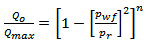 | (17) |
Where n represent the type of flow; 0.5 for turbulent flow and 1 for laminar flow.
2.6. Tubing Performance Relation (TPR)
The tubing performance or outflow performance represents the vertical flow along the tubing and shows the performance of the well in producing from bottom-hole to the surface. It shows the relationship between the flow rate in tubing and the flowing bottom-hole pressure, and is affected by pressure losses experienced due to restrictions in tubing from chokes, valves and connections. Several methods have been proposed to calculate the bottom-hole pressure of a flowing gas well as it is usually not practical to obtain this pressure directly using a pressure gauge at the bottom of the well. The least accurate method is the Average Temperature and Deviation Factor method. Poettmann’s method also uses a constant temperature but uses a compressibility factor value that varies with pressure making it more accurate and realistic than the Average Temperature and Deviation Method. The Cullender and Smith method uses the least number of assumptions and is widely considered as the most accurate.[10] explained that the Cullender and Smith method is more rigorous than the other methods and “is applicable over a much wider range of gas-well pressures and temperature” since it “makes no simplifying assumptions for the variation of either temperature or Z-factor”. The Cullender and Smith method provides a functional relationship between the well flowing bottom-hole pressure (Pwf) and the wellhead pressure (Pwh) as shown in equation 18.  | (18) |
where ‘Qwell’ is the well flow rate, ‘Twf’ the well bottom-hole temperature, ‘Twh’ the wellhead temperature, ‘depth’ the depth of the producing formation from surface, ‘ID’ the inner diameter of the tubing, ‘γg’ the specific gravity of the gas, ‘Ppc’ the critical pressure of the gas, and ‘Tpc’ the critical temperature of the gas.Similarly, pressure gradient charts are available in literature and the pressure gradient is related to outflow for outflow performance analysis. A combination of an inflow performance curve (IPR) and a tubing performance curve (TPR), generally identifies the flow rate and corresponding flowing bottom-hole pressure at a particular reservoir pressure and tubing parameters such as tubing size and wellhead pressure. The deliverability or instantaneous flow rate can then be said to be this combination of the reservoir performance (inflow) and the tubing performance (outflow).
2.7. Prediction of Production and Recovery as a Function of Reservoir Time
Successful evaluation of the exact value of average reservoir pressure per the producing capacity or deliverability is essential for effective resource management. The period to put the well on artificial lift (gas lift) as a function of decline in production capacity relative to the reservoir time is crucial for effective economic analysis of the field. The incremental time required to support incremental cumulative production is given by equation 19. | (19) |
 | (20) |
Hence the cumulative production is given by  | (21) |
2.8. Production Optimization by Artificial Lift
During the life of a producing field, static reservoir pressure may not be in adequate amount to lift economic flow-rates through the wellbore and overcome surface pressure restrictions. Artificial lift systems objective is to reduce bottom hole flowing pressure, net hydrostatic gradient and increase flow rate by injecting gas lift to the down hole produced fluids. Numerous articles related to flow and artificial lift can be found in literature. A few of these examples are cited in the references[11, 12, 13, 14]. As reservoir conditions change with time, artificial lift quantities (gas lift flow, compressor power, pump head, or pump strokes) have to adjust in order to maintain proper fluid production. A continuous depletion of reservoir pressure will cause the bottom hole flowing pressure level sufficiently low as to make the conventional lifting (spontaneous production) inefficient and uneconomic.
3. Results and Discussions
3.1. Hydrocarbon Recovery and Optimization by Artificial Lift
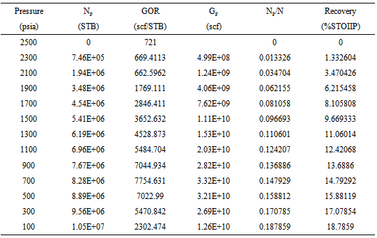
During the life of a producing field, static reservoir pressure may be inadequate amount to lift economic flow-rates through the wellbore and overcome surface pressure restrictions. A continuous depletion of reservoir pressure will cause the bottom hole flowing pressure level sufficiently low as to make the conventional lifting (spontaneous production) inefficient and uneconomic. As pressure continues to decline below the bubble point pressure there is a corresponding evolving and production of gas precipitating the reservoir into depletion as shown in (Fig. 4). The amount of hydrocarbon that can be recovered at any forecasting pressure (Np and Gp) can be easily determined. At abandonment pressure of 100psia, there is only about 18.7% of the stock tank oil initially in place which can be recovered through conventional lifting (Fig. 5). This information is particularly important for the quick response of surface facilities by artificial lift to handle production in a more suitable and economical advantage. Through the artificial lift, the reservoir pressure is kept constant, or there is some compensation in the pressure drop due to production.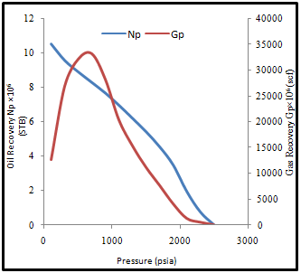 | Figure 4. Production performance as a function of decline pressure |
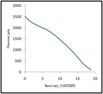 | Figure 5. Average reservoir pressure as a function of cumulative oil production |
3.2. The Solution Gas Oil Ratio and Average Gas Oil Ratio
Fig. 6 shows the relation between solution gas oil ratio (Rs) and the average gas oil ratio Rav calculated against reservoir pressure. The Rav is increasing to a maximum value of about 4003 scf/STB at reservoir pressure 700psia. The increasing gas oil ratio is fairly responsible for the low recovery as in the case studied since there is a corresponding increase in gas mobility reducing oil mobility. This is attributed to larger number of gas bubbles as also indicated by[15]. 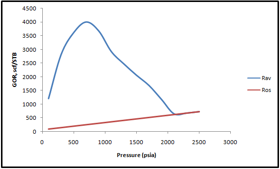 | Figure 6. Produced and solution gas oil ratios as a function of decline pressure |
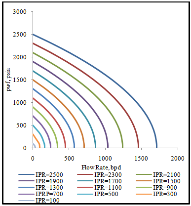 | Figure 7. Fetkovich saturated future IPRs |
3.3. Performance of the Reservoir (IPR)
The performance of the reservoir at any time in the future is crucial in the resource management. The IPR describes the two phase flow in porous medium by Fetkovich model at any average reservoir pressure (Fig. 7). The IPR is established by plotting the gross flow rate at different values of bottom hole flowing pressure. The maximum flow rate obtainable from the analysis is about 1710 bpd. All IPR curves are parallel to each other. The well potential decreases with the decrease in reservoir pressure. The intercept IPR curves with y-axis gives the average reservoir pressure. For the case considered the inflow mobility (ʎ) of the reservoir as a function of formation pressure (pwf) is given as ʎ (pwf) = 7E-08pwf2 + 0.0002pwf + 0.6. This confirms the validity of solution gas reservoirs that below the bubble point that their productivity is not constant as supported by[16]. The function makes determination of any future inflow mobility feasible.
3.4. Effect of Tubing String on Flow Capacity
The size of the production tubing can play an important role in the effectiveness with which the well can produce liquid[17]. There is an optimum tubing size for any well system[18]. Smaller tubing sizes have higher frictional losses and higher gas velocities which provide better transport for the produced liquids. Larger tubing sizes, on the other hand, tend to have lower frictional losses, pressure drops due to lower gas velocities and in turn lower the liquid carrying capacity[17]. Too large tubings will cause a well to load up with liquids and die[18]. (Fig. 8) is plot of the outflow performance relationship (OPR) of the various tubing sizes superimposed on the IPR curves. It is observed that the smaller size tubings have excessive frictional losses with low production rates thereby restricting production. Four larger size tubings (2", 2½", 3" and 4") are considered to be the better candidates to start producing the well. However, the 4" tubing exhibits the lowest frictional loss which might cause the well to load up with liquids and die too early. The 2½" tubing gives a much more reasonable frictional loss as compared to that of 4" and 2" tubings with an equilibrium production rate of about 1200 bpd and an equivalent bottom-hole flowing pressure of about 1350 psi see (Fig. 8).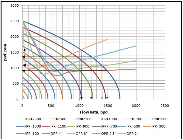 | Figure 8. Plot of IPRs and OPRs for the various tubing sizes |
The point of intersection of the well flow rate and the flowing bottom hole pressure and the well tubing performance gives operating points of the various tubing sizes are shown in Table 2. 2½" tubing was chosen to produce the reservoir from the initial average reservoir pressure of 2500 psia at a GOR of 721 scf/STB up to about 1700 psia with production capacity of 1200bpd. Beyond this point appropriate velocity string would be needed.| Table 2. Equivalent flow capacities of larger tubing sizes |
| | Tubing size (inches) | Bottom-hole pressure (psia) | Producing capacity, (bpd) | | 2” | 1550 | 1040 | | 2.5” | 1350 | 1200 | | 3” | 1050 | 1300 | | 4” | 900 | 1485 |
|
|
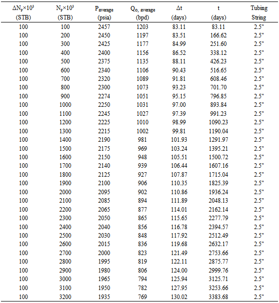
3.5. Forecasting Production and Recovery at Any Future Reservoir Time
Predicting the average reservoir pressure at which the producing capacity will decline to leading to abandonment is very crucial. The reservoir development, planning and successful economic evaluations depends on this data and its availability as a function of time is equally important. The time to place the well on artificial lift and time to install pump or compressors when certain producing capacities can no longer be met is very necessary[16]. To do this the incremental oil recovery ΔNp and the corresponding average pressure Pavg are determined from (Fig. 9). The average pressure is then applied on the (Fig. 10) to determine the corresponding average equivalent production capacity Qoavg. The incremental time Δt, the total time t and the cumulative production Np are determined using equation 19, 20 and 21 respectively. 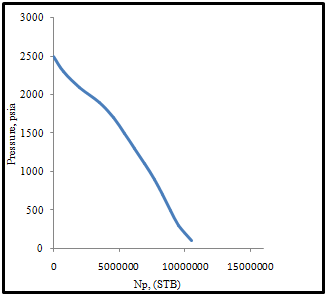 | Figure 9. Average reservoir pressure as a function of cumulative oil production |
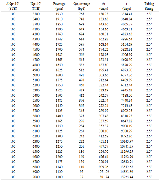
The result of the performance of the field is shown in (Fig. 11). The flow capacity of the field reaches 77 bpd at about 15925 days. Beyond this point pumping will start to optimize the production levels. For detail of the performance analysis see appendix 3. The distribution of the average reservoir pressure over time is shown in (Fig. 12). The reservoir pressure depletion continues up to a region of about 1100 psia. The cumulative oil produced at the abandonment is approximately 7000000Mstb.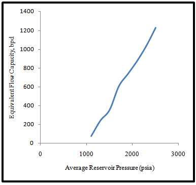 | Figure10. Equivalent flow capacity as a function of decline pressure |
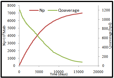 | Figure 11. Production performance as a function of time |
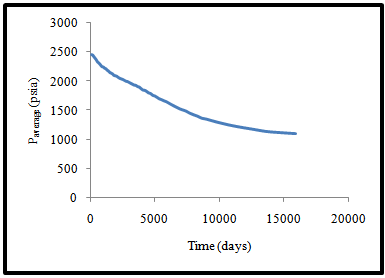 | Figure 12. Average reservoir pressure as a function of time |
4. Conclusions
From the analysis in this paper it can be concluded that saturated-gas drive reservoirs are best candidates for secondary recovery applications due to their low ultimate recovery, about 18% of STOIIP for the case considered. This is explained in the fact that as pressure declined rapidly gas mobility becomes lager with reducing oil mobility due to increasing oil viscosity and hence decreasing oil permeability leading to high gas-oil ratio. Again it has been confirmed that the productivity index also know as mobility index below the bubble point ceases to be constant. It is observed that the outflow performance of a well is largely proportional to the tubing size. The smaller size tubings have excessive frictional losses with low production rates thereby restricting production. Large size tubing exhibits the lowest frictional loss yet their use might cause the well to load up with liquids and die too early. The 2½" tubing gives a much more reasonable frictional loss as compared to that of 4" and 2" tubings with an equilibrium production rate of about 1200 bpd and an equivalent bottom-hole flowing pressure of about 1350. From the IPR analysis the maximum inflow rate obtainable is 1710bpd with an outflow rate of 1200bpd. The flow capacity near abandonment reaches 77bpd at about 15925days with cumulative oil produced estimated at 7MMstb. Combination between material balance equation (Muskat model), the Fetkovich inflow performance relationship model of flow through porous medium and the tubing outflow performance relationship makes an easily forecasting oil production rate. The case considered set out the theoretical framework for the evaluation of the performance and future prediction of saturated gas drive reservoirs.
Appendixs
Appendix 1: Fluid Property Data
 |
| |
|
Appendix 2: Results of the Muskat Primary Prediction Method for the Reservoir
 |
| |
|
Appendix 3: Result of Performance as a Function of Time
 |
| |
|
Appendix 3 Result of Performance as a Function of Time continued
 |
| |
|
References
| [1] | Cole, F., 1969 Reservoir Engineering Manual. Houston: Gulf Publishing Company, 1969. |
| [2] | Tarek, A. 2010. Reservoir Engineering Handbook. Fourth Edition, Doi: 10.1016/C2009-0-30429-8, Gulf Professional Publishing, 30 Corporate Drive, Suite 400, Burlington, MA 01803, USA |
| [3] | Craft, B. C. and Hawkins, M. F., 1960. (revised by Terry, R. E.), Applied Petroleum Reservoir Engineering, Second Edition. Prentice hall PTR Englewood Cliffs, NJ 07632, 1991 |
| [4] | Bimpong, B. O. and Broni-Bediako, E. 2012. Theoretical Design Consideration of Artificial Lift and Tubing String for Solution Gas Drive. VOL. 2, NO. 5, June 2012 ISSN 2225-7217 ARPN Journal of Science and Technology |
| [5] | Bendakhlia, H. Aziz, K. and. Stanford U., 1989. Inflow Performance Relationships for Solution-Gas Drive Horizontal Wells. Doi:10.2118/19823-MS, SPE 19823 |
| [6] | Fetkovich, M. J., “The Isochronal Testing of Oil Wells,” SPE Paper 4529, presented at the SPE 48th Annual Meeting, Las Vegas, Sept. 30–Oct. 3, 1973. |
| [7] | Prado, M. 2008. Two Phase Flow and Nodal Analysis. MSc Lecture Material. African University of Science and Technology, Abuja. 1 -568. |
| [8] | Vogel, J. V., “Inflow Performance Relationships for Solution-Gas Drive Wells,” JPT, Jan. 1968, pp. 86–92; Trans. AIME, p. 243. |
| [9] | Ilk, D., Camacho-Velázquez, R., and Blasingame, T.A., SPE, 2007. Inflow Performance Relationship (IPR) For Solution Gas-Drive Reservoirs -Analytical Considerations SPE Annual Technical Conference and Exhibition held in Anaheim, California, U.S.A., 11–14 November 2007, SPE 110821. |
| [10] | Lee, J. and Wattenbarger, R., Gas Reservoir Engineering, SPE, 1996 Volumetric Gas Reservoirs. Natural Gas Reservoir Engineering, John Wiley and Sons, 1984. 4. |
| [11] | Economides M.J. et al. (edited by) (1998) Petroleum well construction, Chichester-New York, John Wiley. |
| [12] | Economides M.J., Nolte K.G. (2000) Reservoir stimulation, Chichester, John Wiley. |
| [13] | Dusterhoft R.G., Chapman B.J. (1994) Fracturing high permeability reservoirs increases productivity, «Oil & Gas Journal», June. |
| [14] | Mukherjee H. (1999) Fractured well performance. Key to fracture treatment success, «Journal of Petroleum Technology», March, 54-59. |
| [15] | Stewart, C.R. Hunt, E. B., Schneider F. N., Geffen, T. M. and Berry, V. J. 1954. The Role of Bubble Formation in Oil Recovery by Solution Gas Drives in Limestones, Trans., AIME, 201. |
| [16] | Jahanbani, A., Shadizadeh, S. R. 2009. Determination of Inflow Performance Relationship (IPR) by Well Testing. Petroleum Society, Canadian International Petroleum Conference, Paper 2009-086 |
| [17] | Lea, J. F., Nickens, H. V., and Mike, R. 2008. Gas Well Deliquification. Second Edition, Gulf Professional Publishing, 30 Corporate Drive, Suite 400, Burlington, MA 01803, USA. 588. |
| [18] | Beggs, D. 2003. Production Optimization Using Nodal Analysis. Second Edition, OGCI and Petroskills Publications, Tulsa, Oklahoma. 150 - 153. |
 Abstract
 Reference
 Full-Text PDF
 Full-text HTML