-
Paper Information
- Previous Paper
- Paper Submission
-
Journal Information
- About This Journal
- Editorial Board
- Current Issue
- Archive
- Author Guidelines
- Contact Us
Modern International Journal of Pure and Applied Mathematics
2017; 1(3): 46-49
doi:10.5923/j.mijpam.20170103.02

Second Note on the New Shape of S-Convexity
 Abstract
 Reference
 Full-Text PDF
 Full-text HTML
Marcia R. Pinheiro
IICSE University, USA
Correspondence to: Marcia R. Pinheiro, IICSE University, USA.
| Email: |  |
Copyright © 2017 Scientific & Academic Publishing. All Rights Reserved.
This work is licensed under the Creative Commons Attribution International License (CC BY).
http://creativecommons.org/licenses/by/4.0/

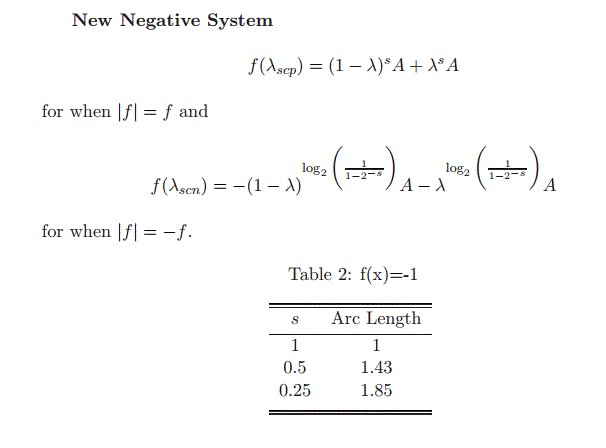
In this note, we copy the work we presented in Second Note on the Shape of S-convexity [1], but apply the reasoning to one of the new limiting lines, limiting lines we presented in Summary and Importance of the Results Involving the Definition of S-Convexity [2]. That line was called New Positive System in Third Note on the Shape of S-convexity [3] because, on that instance, the images of the points of the domain had been replaced with a positive constant, which we called A. This is about Possibility 2 of Summary and Importance of the Results Involving the Definition of S-Convexity. We have called it  in Summary and Importance of the Results Involving the Definition of S-Convexity, and New Positive System in Third Note on the Shape of S-convexity. The second part has already been dealt with in Second Note on the Shape of S-convexity. In Second Note on the Shape of S-convexity, we have already performed the work we performed in First Note on the Shape of S-convexity [4] over the case in which the modulus does not equate the function in the system
  from Summary and Importance of the Results Involving the Definition of S-Convexity. This paper is about progressing toward the main target: Choosing the best limiting lines amongst our candidates.
Keywords: Analysis, Convexity, Definition, S-convexity, Geometry, Shape
Cite this paper: Marcia R. Pinheiro, Second Note on the New Shape of S-Convexity, Modern International Journal of Pure and Applied Mathematics, Vol. 1 No. 3, 2017, pp. 46-49. doi: 10.5923/j.mijpam.20170103.02.
1. Introduction
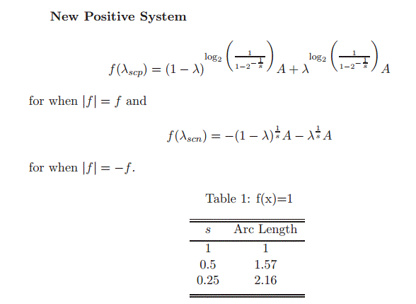 | Figure 1. Third Note, page 736 |
 | Figure 2. Third Note, page 736 |
2. Continuity
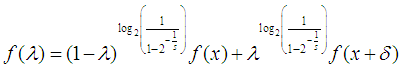
- We now prove that the function
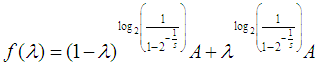 | (1) |
 is continuous, given that
  and
and  . A is a constant, therefore could be seen as a constant function, and the constant function is a continuous function.
 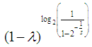 is continuous due to the allowed values for
  and
and  .Making
  and
and  in (1), we get the graph below:
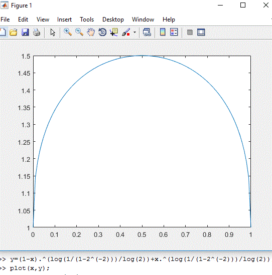 | Figure 3. Maple Plot |
 is
is  , that is, is smooth (see [6] and [7]).
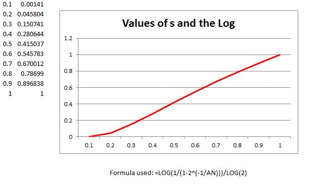 | Figure 4. Value of s |
 convexity limiting line use more than 100% or 100% split between the addends, given that
 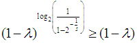 and
and  (we are using the non-negativity of the function here, so
  , but also [9]), we know that the limiting line for
  convexity lies always above or over the limiting line for convexity, with two points that always belong to both the convexity and the
  convexity limiting lines (first and last or
  and
and  ).We now have then proved, in a definite manner, that our limiting line for
  , first part, is smooth, continuous, and located above or over the limiting line for the convexity phenomenon. Our
  convexity limiting line should also be concave when ‘seen’ from the limiting convexity line for the same points ((
 ) and
) and  )) (taking away the cases in which
  or
or  ).
).3. Conclusions
 and
and  are equally acceptable as extensions of the phenomenon Convexity. Notwithstanding, one must remember that the names remain the same (
 and
and  ), but we have in much modified the original definitions that appear in association with them. Throughout the years we have even completely discarded the original definition associated with
  ([8],[9]). We are then left with three possibilities to choose from: Not only our
  and
and  , but also the more geometrically unpleasant, but more analytically welcome, couple formed from the second part of the New Positive and the first part of the New Negative systems [10].We must say that we did not find an ideal match, a match that would bear both analytical and geometrical perfection. The main issue is that we are looking for a single analytical shape that will satisfy both negative and non-negative functions, if possible, something that somehow connects to both the analytical and the geometrical definition [11] of convexity, and will still represent a geometrical distance that is equal in terms of both the
  convexity and the convexity line for both parts of the definition (non-negative and negative). If we were looking into increasing the scope of the line to the upper part on the non-negative side and to the lower part on the negative side, we would not have the same difficulties...Considering the simplest case, of a straight line on a 45-degree angle with the horizontal axis, we would have to move the line that describes the function and the limiting line to the second quadrant, and therefore we would have to mess up with our domain variable, horizontal change, and we then would have to move the set to the third quadrant, and therefore we would have to mess up with our image variable, vertical change. On the last move, it is simply going down the Cartesian Plane, so that we would have to subtract something from the function itself. That would lead to an undesirable algebraic shape straight away, since we would lose in terms of the meaning of the factors that mark our percentage in Convexity.That was thinking as in Vector Algebra, but notice that the fact that the function changes sign will make the inequality change direction, and that is a lot of trouble.It looks like preserving that meaning will cost us somewhere: geometrical aspect, algebraic aspect, complexity of the calculation, and so on. Most of us would privilege calculation, easiness, over perfect geometric match between non-negative and negative parts of the function.