I. Introduction

In [2], we have decided to keep the name and replace the previous class with a new version of it, which would be one of our possible definitions, as for [4].

So far, we have:

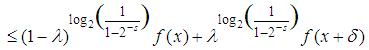
Definition 1. A function , where , is told to belong to if, for each we select, and for all of them, the inequality

Definition 2. A function , where , is told to belong to if, for each we select, and for all of them, the inequality

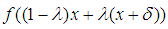
Remark 1. If the inequalities are obeyed in the reverse¹ situation by , then is said to be concave.

We are now going to concentrate only on the pieces of the definition that we have not yet proven in [3].

2. Continuity

We now prove that the function

is continuous through a few theorems from Real Analysis.

We know that both the sum and the product of two continuous functions are continuous functions (see [5]). Notice that is continuous, given that and . and are constants, therefore could be seen as constant functions, which are continuous functions. 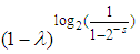is continuous due to the allowed values for and .

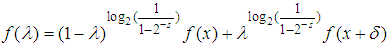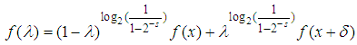
Notice that is , that is, is smooth (see [6]).

Because the coefficients that form the convexity limiting line use 100% split between the addends and form straight lines and the coefficients that form the convexity limiting line use more than 100% or 100% split between the addends, given that and (we are using the negativity of the function here), we know that the limiting line for convexity lies always above or over the limiting line for convexity, and contains two points that always belong to both the convexity and the convexity limiting lines (first and last or and ().

We now have then proved, in a definite manner, also in the shape of a paper, that our limiting line for the convexity phenomenon is smooth, continuous, and located above or over the limiting line for the convexity phenomenon. Our convexity limiting line should also be concave when seen from the limiting convexity line for the same points (taking away the cases in which ).

3. Arc Length

Arc length is defined as the length along a curve,

where dl is a differential displacement vector along a curve (see [7]).

In Cartesian coordinates, that means that the Arc Length of a curve is given by

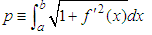whenever the curve is written in the shape .

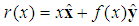Our limiting curve for convexity could be expressed as a function of in the following way:

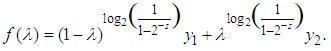In deriving the above function in terms of , we get:

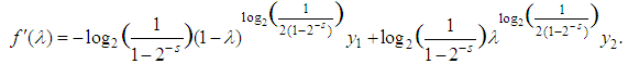With this, our arc length formula will return:

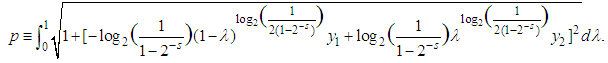We will make use of a constant function, and we know that every constant function is convex, therefore also convex (for every allowed value of s), to study the limiting line for convexity better.

We choose to work with (this function is suitable because ).

We then have:

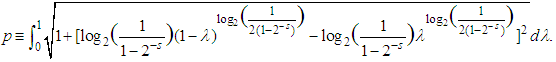Notice that indeterminate and .

Notice that 0.25 will become 0.09 when raised to and its supplement through the formula , 0.75, will become 0.6.

In convexity, our results would have been 0.25 and 0.75 instead, that is, 64% and 20% less in negativity is gotten with convexity, respectively.

We now calculate the area under the curve by hand because Maple could not compute it inside of an acceptable time interval: We notice that the vertex of the graph that represents the function we are interested in is located on (0.5; 1) in both cases. We can then draw a triangle on both sides of the space we are interested in, and find an approximation to our target area. After that, we can subtract an approximation to the piece of the triangle we cannot consider. From eye observation, we can tell that the second leaf is about half of the first, so that whatever we put for the first, we just halve it for the second.

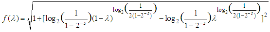
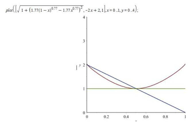Figure 1. Maple Plot, s=0.5

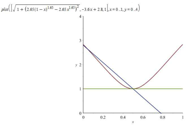Figure 2. Maple Plot, s=0.25

The top triangle of the first graph has base of size 0.5 and height of size 1. The top triangle of the second graph has base of size 0.5 and height of size of about 1.8. Base times height will then be equal to 0.5 and 0.9.

The area of the just-mentioned triangles is then 0.25 and 0.45, but we have two of each. We then have 0.5 and 0.9, respectively, as areas for the top part of each one of the graphs, but we still have to take away the leaves.

Upon using the grid option from Maple, we concluded that it would be fair saying that approximately 12.5% of the triangles from the first graph would be committed to being above the curve, so that we would have 87.5% of the original area left only. That would mean 87.5% of 0.5 or 0.4.

Similar reasoning leads to 92% of the second set remaining of interest to us, that is, 92% of 0.9 or 0.8 (approximation).

Now we have to add the rectangle we skipped when doing that, which is what comes before the base line we drew: A rectangle of one unit of length and one unit of height, and therefore a rectangle of area equal to 1.

To get the right approximation, we need to now put it all together: For the figure 1, it will then be 0.4+1=1.4, and, for Figure 2, it will be 0.8+1=1.8.

We finish this section with a table² containing three of the possible values for s and their respective arc lengths (good approximations. Only the first value is precise) for the situation in which is replaced with -1 in the arc length formula:

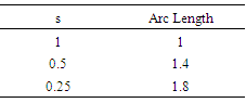
4. Maximum Height

The maximum height of the convexity limiting curve is reached when if is constant and because the first derivative of the function describing the limiting line gives us zero for and changes sign from positive to negative.

5. Comparison of Results

Our calculations in [3] had made use of instead of . Today we used Maple and for when we have modulus equating function and exponent being only s. Our results were:

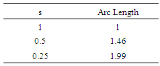When we used exponent instead for the case in which the modulus does not equate the function, we got, for , this time through Maple, the following table:

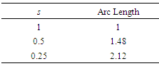
6. Conclusions

Our studies on length were, so far, based on rough approximations. In this paper, we could use Maple to build the table of lengths for two situations, and those were our best matches in terms of algebraic form and all else. We measured length for the case of modulus equating function and exponent s and for the case modulus not equating function and exponent .

We have studied alternatives to the exponent because it seemed that there was non-negligible discrepancy between the case in which the modulus equates the function and the case in which it doesn't.

The replacement has been thought of because ideally we would have the same height all the way through for the limiting curve in both the negative and the non-negative case, but such fact was not being verified with the previous definition, as seen on [4].

We definitely needed to keep the points where at the same height.

That is why our only possible alternative would be the limiting line containing the log, as seen in [4].

Upon considering the figures attained for in the system containing the exponent s for the case in which the modulus of the function does not equate the function, and comparing those with the figures we get for and exponent s, studied here under the light of Maple, we notice that the values are compatible enough.

Maple could not calculate the integral for the case in which we have the log, but our rough approximations make us think that the figures are compatible enough and our rough approximations gave us figures that were similar enough for the case in which the exponent was when the results attained with Maple are considered.

Our best choice could be and s because the algebraic form is nicer, the calculations are easier (Maple could calculate for for instance), and the match is instinctive.

We started thinking of a new shape because of the discrepancies found in terms of the tables involving both the negative and the non-negative functions for these shapes however.

If we consider basic values, such as , , , and , the results of our calculations show us that we should adopt s and log as exponents instead.

We worry about the distance encountered between the limiting line for S-convexity and the line for convexity, as seen in [4].

When we write as exponent, we should have and this distance should be the same as the distance between and 1. This distance is approximately 0.41. We can also call it now, thanks to [2]. When we have exponent , we should have , and the distance should be the same as the distance between and 1, and that is 0.5.

When we write the log as exponent, and consider the negative function, we get 0.41 once more.

In this case, the ideal couple is s and log or the New Negative from [4]. However, we must still analyze the case New Positive in full.

Notes

1. Reverse here means `>', not `≥'.

2. The first value for Arc Length in the table has been attained through simple substitution in the formula.