Brian E. Usibe, Oleksandr V. Menshykov
School of Engineering, University of Aberdeen, Aberdeen, Scotland, UK
Correspondence to: Brian E. Usibe, School of Engineering, University of Aberdeen, Aberdeen, Scotland, UK.
| Email: |  |
Copyright © 2021 The Author(s). Published by Scientific & Academic Publishing.
This work is licensed under the Creative Commons Attribution International License (CC BY).
http://creativecommons.org/licenses/by/4.0/

Abstract
Cracks in elastic media vary significantly, depending on the nature (frequency, direction and magnitude) of the external load as well as the material properties. Therefore, the methods of determining the fracture parameter (Stress Intensity Factor) depends on the crack geometry, which also influences the choice of elements and mesh generation in Finite Element Analysis. In this paper, the Griffith centroid crack is modelled in 3D Finite Elements under harmonic loading. The numerical results of Stress field variables and displacement jumps are compared in order to determine the suitable and reliable method for determining appropriate dynamic SIF of the through-thickness crack. The accuracy and variations of the results were only dependent on the mesh refinement of the isoparametric hexahedral element in the vicinity of the crack tip. The obtained result, which agrees with literature also establishes the validity of the model for both methods of solving mode I fracture dynamic problems, numerically, irrespective of the mesh and element type. For both methods adopted for the determination of SIF, the plane strain condition was satisfied.
Keywords:
Stress Intensity Factor, Fracture dynamics, Harmonic loading, Finite Elements
Cite this paper: Brian E. Usibe, Oleksandr V. Menshykov, Evaluation of Dynamic Stress Intensity Factor of Griffith Crack Using the Finite Element Method, International Journal of Mechanics and Applications, Vol. 10 No. 1, 2021, pp. 1-10. doi: 10.5923/j.mechanics.20211001.01.
1. Introduction
The understanding of the dynamic responses of fractured elastic media subjected to different loading conditions is important and of great interest to a variety of scientific and engineering fields where structural integrity is needed. The responses of materials under loading are significantly influenced by the presence of cracks and since flaws are essentially unavoidable, it is often necessary to assume a crack of some given size will be present in a material. According to [1], the discrepancy between the observed fracture strength of crystals and the theoretical cohesive strength was due to the presence of flaws in brittle materials. Though this theory is applicable to a perfectly brittle material such as glass, Griffith’s ideas formed a base to understand the fracture mechanism in metals. The presence of defects serve as stress concentration regions and can significantly decrease the overall lifetime of the structures resulting in sudden failure under small loads, which puts human health and life at risk. There is also the increase in the cost of maintenance and consequential costs of repairs and loss of revenue for any failures that occur [2].It is necessary to predict how cracked engineering materials will behave under loadings, as they tend to fail under very small unexpected stresses. Therefore, there is need to develop suitable models and procedures that would form the basis for assessing the integrity, sensitivity and standards of engineering structures, thereby remedying the risk of deterioration and subsequent failures of these structures due to flaws and crack-like defects. The understanding of the failure mechanism, which is the description of technical failure modes resulting from degradation of components due to in-service combined with fabrication errors lead to the concept of Fracture Mechanics. Fracture Mechanics, as an engineering field deals with the propagation of cracks in materials. It studies the failure of solids from crack initiation stage to propagation, then to fracture. It finds application in all engineering fields where engineering materials are used including; investigation of critical crack sizes in aircraft wings, creep rupture studies of concrete, brittle fracture of cargo ships, etc. The relationship between applied loads and the size and location of a crack in a structure can be determined with the help of Fracture Mechanics solutions, which plays a role in the prediction of the rate of the crack growth [3]. The rate of cracking can be correlated with Fracture Mechanics Parameters such as the Stress Intensity Factor and the critical crack size for failure can be computed if the fracture toughness, Kc is known. Fracture Mechanics quantifies the critical combinations of the three variables; the applied stress, crack size and the fracture toughness for the determination of material suitability, contrary to the traditional strength of material approach, which assumes that a material is adequate if its strength is greater than the expected applied stress. In such an approach, a safety factor on stress, combined with minimum tensile elongation requirements on the material may be introduced to guard against brittle fracture. Whereas, Fracture Mechanics has an important additional structural variables; crack size and the fracture toughness, which replaces strength as the relevant material property [3]. The crack size and shape, the specimen geometry and loading, along with material fracture toughness (a measure of a material with pre-existing crack to resist fracture) can be used to determine the ability of the material to resist fracture [4]. The importance of related geometric correction factors for compliance in the determination of Stress Intensity factor was also described in [5]. This is why it important to accurately determine the fracture parameters, especially when it is obvious that under harmonic loading, the closure effect of the opposite crack faces significantly alters the distribution of the Stress state in the vicinity of the crack-tip [6]. The field of Mechanics can be classified as Analytical Mechanics, Experimental Mechanics and Computational Mechanics. Due to the enormous progress in Computer Technology and numerical techniques in the recent years, the use of computational method has gained more importance and popularity for complex industrial problems which are limited by analytical methods [7]. The complexity of dynamic loads, crack geometry and the heterogeneity of material properties can only be handled by computational methods of fracture studies. Amongst the three techniques, numerical simulation techniques have become established as a widely self-contained scientific discipline and numerical simulations prove to be best suitable to solve problems of fracture dynamics due to its comprehensive result sets, generating the physical response of the system at any location [8]. Therefore, the numerical method is used in this work for determining the Stress Intensity Factor. Numerical approaches could either be based on field variables or energy balance. However, the authors have adopted the contemporary field variable approach due to its reliability, convenience and simplicity in calculating the desired fracture parameter. One interesting method used in computational and numerical modelling of engineering problems is the Finite Element Method which has found extensive usage and applications in mechanics and fracture dynamics. In the formulation of Finite Element models, discretization is a major technique and requirement, therefore the choice of elements and the development of refined meshes that will fit and define the problem geometry, while satisfying the pre-determined constraints (loading conditions and material properties) is an essential aspect of the FE modelling. With the Finite Element Analysis (FEA), the understanding of the behaviour of a cracked structural component under harmonic loading will be enhanced and the dynamic Stress Intensity Factor (DSIF) which predicts an acceptable crack size and stress levels before propagation occurs can be determined numerically.Below are practical steps for FEA solution to the Fracture Mechanics problem: • We develop/define the model which represents the physical problem of Griffith crack to be solved• Choose a suitable element (isoparametric hexahedral element) for the problem and discretize the domain by forming the corresponding Finite Element Mesh• Refine the Mesh at the crack tip region of the model• Assign the interpolation function to represent the variation (at nodal points) of the field variable over the element• Define the properties of the individual elements according to the physical material/problem• Assemble the element properties to obtain the system equations for the complete network of elements• Apply boundary conditions, constraints and harmonic loading(s) to the model, using the known nodal values of the dependent variables. This completes the description of the physical problem• Obtain the unknown nodal values of the problem at nodal points to check accuracy of results (note: stresses are obtained over an entire element or integration point)• Repeat the computation to obtain all desired unknowns (Displacement fields and stresses at crack tip)• Extract the numerical results using an IDE and then compute the fracture parameter (Stress Intensity factor)The Stress Intensity Factor (SIF), K is the main fracture parameter for the integrity assessment of structures containing cracks. The SIF quantifies the singularity intensity of an elastic crack-tip stress field, which forms the foundation for LEFM and is used to describe the fracture resistance  (known as mode I fracture toughness) of a material. By introducing SIF, the fracture criterion can be formulated [9]. Accordingly, fracture starts when SIF, KI reaches a material-specific critical value,
  (for mode I). Once K is obtained for any mode, elastic crack assessment can be performed. This determination of K is of great engineering importance and it is necessary to calculate K with high accuracy in order to assess the integrity of cracked components precisely. Based on K, it is possible to establish when a material will fracture due to a critical crack length or stress level.
2. Statement of Problem and Finite Element Set up
Consider a 3D linear elastic homogeneous isotropic solid  with properties of steel (Young’s modulus E = 200 GPa, Poisson’s ratio ν = 0.3, density ρ = 7800 kg/m3), having a through-thickness interfacial crack between the half-spaces, under normal tension-compresion harmonic incident wave. The model has been built using Abaqus/CAE with opposite crack faces having an initial “small” opening of 10-6 mm and we assume that only small deformations occur in line with LEFM. The model satisfies the plane strain conditions of crack aspect ratio. Under harmonic wave, the internal crack opens and closes during tensile and compressive phases, respectively. The orientation of the plane strain FEA model for figure 1 is a good representation of the center through-thickness crack specimen behaviour where the thickness is fixed. In practice, this condition is used where the stress state is varying slowly from plane to plane in a deep component. There should be enough material in depth to stabilize and eliminate the through thickness strain. This assumption is useful to characterise the fracture toughness for mode I,
  as is the case of this model.
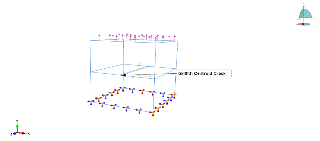 | Figure 1. FE Model of through-thickness crack under loading |
According to fracture mechanics theory, KI is a function of the far-field stress, the crack size, the shape and orientation of the crack as well as dimensions of the specimen. There exist many techniques to determine SIF from FE field variables (stress or displacement). The numerical methods for calculating K can be divided into the field variable methods and the energy release methods. The field variable methods can be further divided into displacement based and stress-based methods [10]. Here, the stress extrapolation and displacement correlation methods have been used to calculate SIF since these methods can be applied to all types of elements. The basic idea of any method used is relating the SIF with the physical quantities (such as stresses, displacements) around the crack front, which have been determined by FE analysis. Stress field variables are obtained at integration points closest to the crack tip and the SIF can be calculated using equation (1) [11] and extrapolated to zero (representing the crack tip).For a mode I through thickness crack-front field in which  and
and  are principal stresses at a node, parallel and perpendicular to crack directions respectively, the stress fields are defined as;
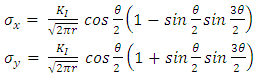 | (1) |
Where the normal stress,  along the crack surface
  is adopted in the calculation of SIF.
  is the relative distance from the crack tip and
  can be obtained;
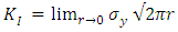 | (2) |
With a plot of  as a function of r, SIF at the crack front can be determined by extrapolation.Similarly, from the displacement field around the crack tip;
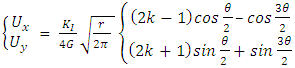 | (3) |
Where  (for plane strain condition),
  is shear modulus, E and
  are the Young modulus and Poisson ratio of the material, respectively. With displacement jumps at nodal positions along the crack plane, SIF is calculated using equation (4). Note that
  along the crack surface
  is adopted in SIF calculation.
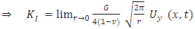 | (4) |
Where  is the shear modulus and
  is Poisson ratio of the material.
  is the relative distance from the crack tip. For mode II crack,
  has an expression like equation (4) with the parallel (x-direction) displacement,
  to replace,
  [12], [13] and [14].Figures 2 shows the Displacement Jump [U] method correlated from two adjacent nodes on the crack faces closest to the crack tip. In the stress extrapolation method shown in figure 3, the SIF is obtained for normal stress components along the crack plane, as
  , which also describes the crack-tip.
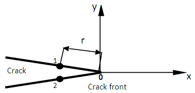 | Figures 2. Displacement Jump |
 | Figures 3. Stress Extrapolation |
The idea of the displacement jump method is to find the displacements of the points located on the top and bottom half-spaces at the interface across the crack and the dynamic Stress Intensity Factor based on the expression of the displacement field in the vicinity of the crack tip. Hence, the single displacement jump is the relative displacement between points 1 and 2 located at the same distance, r [15]. The displacement jump [U] is obtained at unique nodal as follows; | (5) |
On the other method, the applied stress of interest is considered in the normal tension-compression loading case for the incident wave. It should be noted that stresses are obtained at Integration Points in FEM and then extrapolated to nodal positions. From equations (1), there is an inverse relationship between stresses and the distance from the crack front, r. As the value of r approaches zero, the value of stresses increase significantly. However, stresses become infinite if the problem is solved at the crack tip (r = 0), which is impossible in real life as no material can sustain infinite stresses. As a result, the region of plastic deformation must be assumed to be negligibly small compared to all characteristic dimensions of the body [9]. Under these circumstances, it can be assumed that the area of the plastic zone is controlled by the K-dominated field. The fracture will commence when values of stresses concentrated at the crack tip are high enough to cause the propagation of the crack. Therefore, crack propagation starts when the Stress Intensity Factor, K reaches a certain critical value KC of any material.
3. Numerical Results and Discussions
Mesh and Element GenerationIn this paper, the FE model of the through-thickness crack (figure 4) is based on hexahedral mesh, generated using C3D8R (an 8-node linear brick, reduced integration, hour glass) isoparametric elements, which usually provides a solution of good accuracy at less cost (Abaqus/CAE 6.14-1). It best identifies the characteristics of this model, being a three-dimensional continuum (solid) cube using the explicit analysis (for dynamic stress and displacement) that provides flexibility in the modelling of different geometries and structures. The presence of stress singularities at the crack tip requires mesh refinement and reduction of element size around that region. This allows for the accurate determination of field variables around the crack front. This can be achieved by a rapid transition from small elements near the crack front to much larger elements in the other parts of the domain where spatial gradient variations are expected [16]. The hexahedral element is also good for the formation of quarter-point elements by collapsing some of the crack-tip nodes for some other complicated geometries.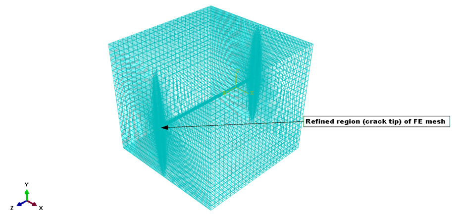 | Figure 4. FE mesh of through-thickness crack |
In the FE formulation, the stress and displacement extrapolation methods have been comparatively used to determine SIF (Mode I) since these methods can be applied to all types of elements (no special crack tip elements are needed). Mesh refinement and sensitivity study are sufficient to approximate the singularity at the crack tip of the FE model for accurate results. The investigation and use of special crack tip elements are suitable for other kinds of crack configuration, especially the elliptical or penny-shaped cracks where there are curvatures and blunt edges. On the other hand, hexahedral elements simply adopts polynomials to interpolate field variables in the FE domain of interest. The basic idea of any method used is relating the SIF with the physical quantities (such as stresses or displacements) around the crack tip, which have been determined by FE analysis. The result FE model is shown in figure 5 with obvious stress concentration can be observed at the crack tip. 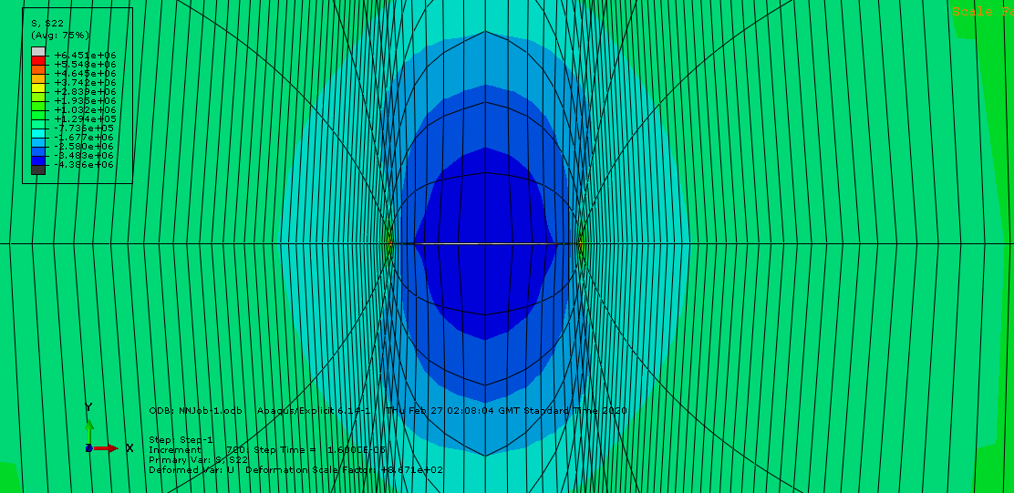 | Figure 5. FE Model result of the Griffith crack |
Harmonic Wave Distribution(i) Dynamic StressBy using the stress extrapolation and displacement jump methods, KI in the vicinity of the crack front is computed for the FE model. The problem is solved for the crack under normal tension-compression loading as shown in the distribution of the applied dynamic stress as a function of time. A harmonic load of frequency ω=2πf is applied as a uniformly distributed pressure to the FE model in the normal direction. The amplitude of the applied load is periodic with step time and initial amplitude using the Fourier function;  | (6) |
The amplitudes  and
and  of the Fourier functions are represented by components of the tractions and displacements, respectively as shown below;
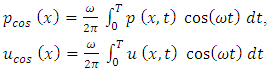 | (7) |
 | (8) |
The incident tension-compression harmonic wave is defined by the potential function; 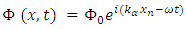 | (9) |
Where  and ω are the amplitude and the frequency of the incident wave, respectively,
  is the generalized wave number given by
  and
and  are the velocities of incident waves in elastic media [6].
 | (10) |
Where λ and µ are lame constants and ρ is the density of the material (in this case steel). The results of the applied load in time and the corresponding stress distribution along the crack plane for a periodic incident wave on the FE model of figure 6 are shown in figures 7 and 8. | Figure 6a. The model at initial loading |
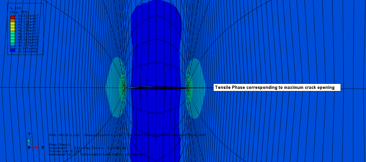 | Figure 6b. The tensile phase |
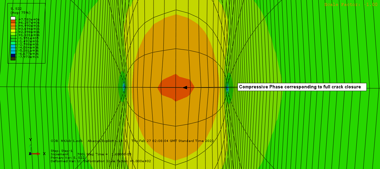 | Figure 6c. The compressive phase |
 | Figure 7. Applied stress in time |
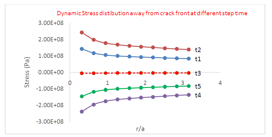 | Figure 8. Dynamic Stress distribution in the crack plane |
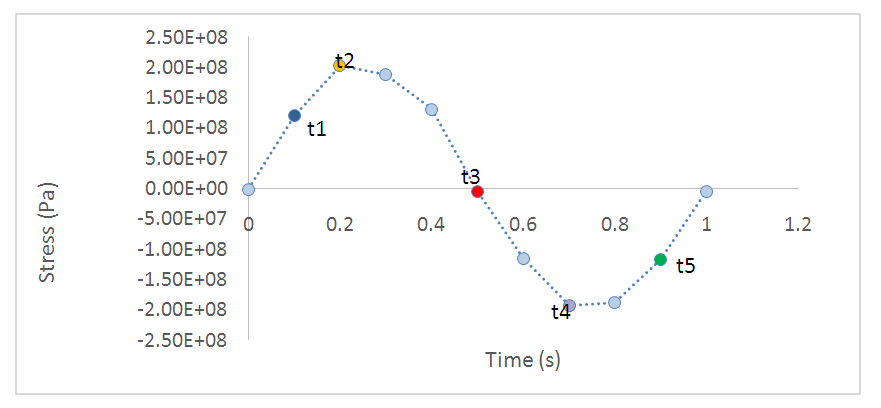
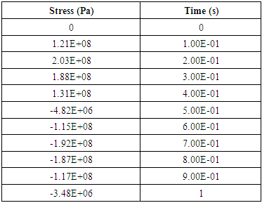
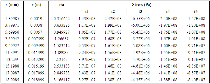
Typical stress distribution around the crack plane are shown with obvious stress concentration observed at the crack tip during tensile phase. With the application of the dynamic normal load, there is an increase in the stress level at the contact region of the crack surface and the model is deformed based on the load increment, with each time step until the complete cycle. The numerical results of stresses and displacement jumps obtained from the FE model are used for the calculation of the dynamic SIFs at the end of each load step.Results of applied stress as a function of time is shown in table 1. The applied stress of interest is considered in the normal Y-directions at a time interval, for selected points away from the crack front at normalised distances. The results were obtained for the normal tension-compression loading case for the incident wave at element number 578.Table 1. Stress in time
 |
| |
|
The results of the dynamic stress distribution along the crack plane at distances, r and a crack size, a are presented in table 2 for selected points depicted as t1, t2, t3, t4 and t5. (See figure 8 for interpretation of results).Table 2. Dynamic stress distribution along the crack plane at different step time
 |
| |
|
The stress distribution away from the crack front is shown in figure 8, for selected points (step time), depicted as t1, t2 (tensile phase), t3 and t4, t5 (compressive phase) with the respective annotation. It can be seen that higher stress amplitude was obtained as the distance towards the crack tip tends to zero, with both tensile and compressive phases. Far away from the front, the dynamic load tends to the static applied value. It should be noted that stresses become infinite if the problem is solved at the crack tip  which is impossible in real life as no material can sustain infinite stresses.(ii) Nodal Displacement JumpSimilarly, the time-dependent nodal displacements being the interconnection points of the elements which also undergo harmonic deformation due to the dynamic loading is shown if figure 9. The displacement output of any node is a function of its global Cartesian coordinate system. The displacement jumps distribution obtained in the FEA is in the normal Y-direction for the pair of selected nodes closest to the crack front at a distance, r. The nodal displacement jumps tends to zero as the crack tip is approached, as seen on the curve obtained from the crack plane.
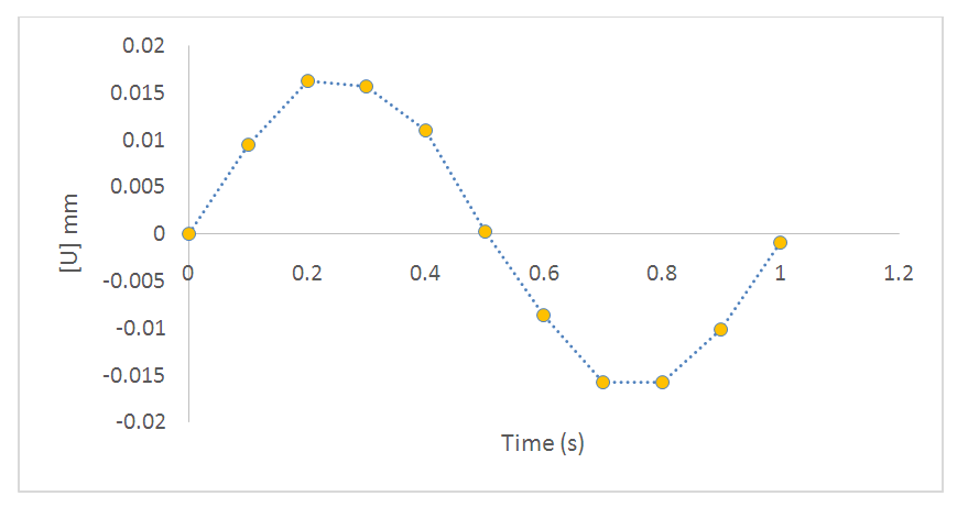 | Figure 9. Distribution of displacement jump as a function of time |
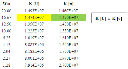
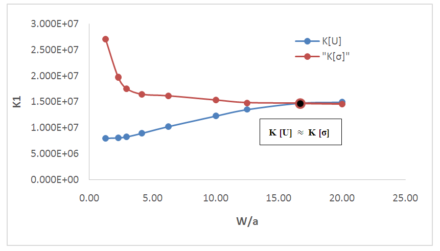
Comparable SIFs for stress fields and Displacement JumpsThe dynamic SIF obtained from the FE results of both stress fields and displacement jumps are comparable as seen in figure 10. The normalised  values obtained for the varying crack aspect ratio shows the plane strain SIF decays gradually towards a constant with varying crack dimension, until a change in crack size and specimen dimension become insignificant to the results (See table 3). It also establishes the validity of the model for both methods of solving fracture dynamic problems, numerically, irrespective of the mesh and element type, where K [U] and K [σ] were calculated Stress Intensity Factors from displacement jumps and stress field of the numerical model. This result corresponds to that in [9], therefore it is valid as first step a solution for fundamental problems of mode I elastodynamic cracks. The solution is of great relevance since all structural members have finite dimensions and cracks are most commonly located within half-spaces and/or through the thickness of solid materials.
Table 3. Stress intensity factor values from both displacement jump and stress field variables
 |
| |
|
 | Figure 10. Variation of comparable SIFs with crack size |
From the numerical results and illustration of the through thickness crack, it was found that an increasing ratio of crack length to specimen width decreases the Stress Intensity Factor and vice versa. Hence, the ratio of crack length to plate width can be used as a design parameter that affects the fracture toughness and as a tool of predicting condition for failure of a structural member.
4. Conclusions
In the FE model, the distributions of normal stress components and displacement jumps for the through-thickness crack located in the center of a 3D homogeneous solid under harmonic loading was obtained and the Stress Intensity Factor, KI for mode I was computed using stress and displacement extrapolation methods, respectively. The variations of K as a function of crack aspect ratio was also analysed. The numerical K obtained from stress field and displacement jumps show both methods of calculating K are comparable for the same crack size and fixed specimen dimension. The results show the validity of the FEA model and both methods can simply be used to determine accurate values of SIFs, irrespective of the element type (so long as mesh refinement is achieved in the crack vicinity), which indicates that the Finite Element Method is reliable and would achieve the correct expectation of results for complex cases when contact interaction is taken into account. In what follows, it is recommended that the Dynamic Stress Intensity Factors for opening mode be computed as a function of varying wave numbers, taking the effects of crack closure into account, which defines the 'true-state' Physics phenomena of the dynamic problem.
Nomenclature
References
| [1] | Griffith, A. A. (1920): The phenomena of rupture and flow in solids. Philosophical Transactions of the Royal Society of London, A221, pp. 163-198. |
| [2] | Daud, R., Ariffin, A. K., Abdullah, S. and Ismail, Al. E. (2012): Applied Fracture Mechanics – Interacting Cracks Analysis Using Finite Element Method. Intech Publishers. |
| [3] | Anderson, T.L. (1995) Fracture Mechanics. Fundamentals and Applications. 2nd edition, Boca Raton, CRC Press. |
| [4] | Carlson, R. L., Kardomateas, G. A. and Graig, J. I. (2012): Mechanics of Failure Mechanism is Structures. Springer Dordrecht Heidelberg New York. Pp 8-9, 13-15. |
| [5] | John U. Arikpo, Michael U. Onuu and Brian E. Usibe (2013): Comparative Study of Stress Intensity Factor of Some Engineering Materials Elixir Chem. Phys. 65: 20096-20102. |
| [6] | O. V. Menshykov and I. A. Guz (2007): Effect of Contact Interaction of the Crack Faces for a Crack under Harmonic Loading. International Applied Mechanics, Vol. 43, No. 7, Pp 809-815. |
| [7] | Schäfer, M. (2006): Computational Engineering – Introduction to Numerical Methods. Springer Berlin Heidelberg, New York. |
| [8] | K. H. Huebner, D. L. Dewhirst, D. E. Smith and J. G. Byron (2001): The Finite Element for Engineers. Wiley-interscience, New York. |
| [9] | Gross, D. and Seelig, T. (2011): Fracture Mechanics with an Introduction to Micromechanics. Springer Heidelberg Dordrecht, New York. |
| [10] | G. Qian, V. F. Gonzalez-Albuixech, M. Neffenger, E. Giner (2016): Comparison of KI calculation methods. Engineering Fracture Mechanics Vol 56, Pp 52-67. |
| [11] | W. D. Callister (2008): Materials Science and Engineering. An Introduction. John Wiley & Sons Inc. Pp 184-232. |
| [12] | Han, Q., Wang, Y., Yin, Y. and Wang, D. (2015): Determination of stress intensity factor for mode I fatigue crack based on finite element analysis. Engineering Fracture Mechanics Vol 138, Pp 118–126. |
| [13] | B. Zafošnik and G. Fajdiga (2016): Determining Stress Intensity Factor Ki with Extrapolation Method. Technical Gazette Vol 23, No 6, Pp 1673-1678. |
| [14] | Zhu, X-K and Leis, B. N. (2014): Effective Methods to Determine Stress Intensity Factors for 2D and 3D Cracks. American Society of Mechanical Engineering. https://doi.org/10.1115/IPC2014-33120. |
| [15] | K. C. Nehar, B. E. Hachi, F. Cazes, M. Haboussi 2 (2017): Evaluation of stress intensity factors for bi-material interface cracks using displacement jump methods. Acta Mech. Sin. Vol 33(6), Pp 1051–1064. DOI 10.1007/s10409-017-0711-6. |
| [16] | Zuo, J., Deng, X. and Sutton, M. A. (2005): Advances in Tetrahedral Mesh Generation for Modelling of Three-Dimensional Regions With Complex, Curvilinear Crack Shapes. International Journal for Numerical Methods in Engineering. 63:256–275. DOI:10.1002/nme.1285. |

 Abstract
 Reference
 Full-Text PDF
 Full-text HTML