Kiplangat C. Kononden
Department of Energy Engineering, Moi University, Eldoret, Kenya
Correspondence to: Kiplangat C. Kononden, Department of Energy Engineering, Moi University, Eldoret, Kenya.
| Email: |  |
Copyright © 2018 The Author(s). Published by Scientific & Academic Publishing.
This work is licensed under the Creative Commons Attribution International License (CC BY).
http://creativecommons.org/licenses/by/4.0/

Abstract
While pursuing the search for a perpetual motion machine I came across something interesting that I would like to present its findings. This paper presents the outcome of experiments done using “Autodesk Inventor Professional” engineering software. A system was designed that contains a pendulum which virtually maintains its maximum displaced position, but appears to be rotating round its pivot, as it is dragged along a circular orbit. Further, the research studied all the resultant torque when revolving the virtual pendulum system. During the experiments, the gravitational forces as well as the centrifugal effects due to axial and orbital rotation are taken into account. However the brunt of air resistant on the system has not been integrated since they are deemed to have negligible effect. Experimental results showed that, damping or friction at pivot  and
and  comparatively shifts the equilibrium of pendulum 1 and 2 from their natural vertical positions. This occurs when the two pendulums are revolved on a circular orbit whose centre is
  Moreover, a shift in the pendulum’s equilibrium induces a resultant torque at pivot
  The findings of these experiments are crucial in the design of a vertical merry go round and any other similar structure that has a revolving pendulum. The other relevant application is in the excavator arm and bucket link performance.
Keywords:
Energy, Pendulum, Equilibrium, Torque, Damping
Cite this paper: Kiplangat C. Kononden, Energy Balance in a Revolving Virtual Pendulum System, International Journal of Mechanics and Applications, Vol. 8 No. 1, 2018, pp. 10-20. doi: 10.5923/j.mechanics.20180801.02.
1. Introduction
A linear pendulum comprises of a mass, or bob, coupled to a rod or rope, that experiences simple harmonic motion as it swings back and forth ideally without friction. The equilibrium position of the pendulum is the position when the mass is hanging directly downward [1]. On the other hand a perpetual motion machine is a machine that in essence has efficiency higher than 100% and therefore can provide a continuous motion even in the case of frictional resistance. Hypothetically perpetual motion machine can do work indefinitely without an energy source. However, this kind of machine is up to now not practical [2, 3, 4, and 5].Referring to a linear pendulum system displaced at an angle  from the equilibrium it is known that the mass or bob accelerates toward the equilibrium position and as it passes through the nadir, it starts slowing down until it reaches position
  and then accelerate back [1]. The pendulum has zero torque at the pivot, when its centre of gravity is placed directly vertical to the pivot. Nonetheless, it increases to maximum as it approaches horizontal position. Usually, the mechanical friction at the pivot brings the pendulum to halt at its lowest possible datum [6]. Figure 1 shows a free body diagram of a linear pendulum as it oscillates after being displaced at an angle
  from the equilibrium position.
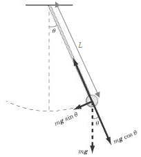 | Figure 1. Free body diagram of a linear pendulum |
The torque  as observed at the pendulum’s pivot is given by the following arithmetical relation [7, 8]:
 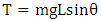 | (1) |
The experiments in this research are far much different from the usual experiments that are meant to study the frictional effects and period variations as the pendulum oscillates [9, 10]. Further, the structure designed in this research contains a pendulum that virtually maintains its maximum displaced position but appears to be revolving around its pivot as it is dragged along a circular orbit.The experiments performed, investigates the resultant motion and torque when the pivot of the pendulum is not fixed but rather exhibits curvilinear motion. The design of the structure used for the experiments is discussed in the following section.
2. Conceptual Design and Theory of the Virtual Pendulum System
2.1. Conceptual Design
Figure 2 show the graphical design concept of the revolving virtual pendulum system drawn using Autodesk Inventor computer program. The central pivot  is hinged to an imaginary external fixed housing frame by use of a radial bearing system. Moreover the central shaft is designed to be accessible for output or input power purposes. At each end of the beam balance rod are the; pivot
  and pivot
  hosting the pendulum rod with the mass at the end. They too are designed to be accessible for output or input power purposes. The beam balance rod is holed and has a mass of 3 kg, while the pendulum rod has a mass of 0.5 kg each. Each pendulum bob has a mass of 5 kg. During the experiment a resistive or a driving torque is applied to each of the three pivots as required. In this research a resistive torque represents an electric generator (dynamo) while a driving torque represents an electric motor.
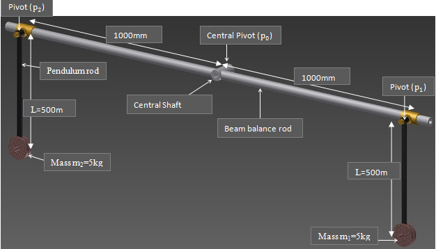 | Figure 2. Graphical representation of the poised virtual pendulum system |
2.2. Theory and Schematic Diagrams
Figure 3 (a), (b), (c) show the schematic diagram of the dynamic virtual pendulum system. In figure 3 (a), the system is at a poised state. Also, the angle of displacement at the central pivot is zero and therefore the system is at an equilibrised position. Conversely the system in figure 3 (b) is at a dynamic state. Even so there is zero resistance torque at the central pivot since the system is at equilibrium. Also noted is that the pendulum remains at its angular position due to zero friction at the hinges which means zero drag force. In figure 3 (c) the system is at a dynamic state. However it experiences a resisting torque due to the inclined nature of the pendulums. As a result to frictions (e.g. electric dynamo) at the pivot 1 and 2 there is a resultant drag force that shifts the angular position of the pendulum. Derived from equation 1, the maximum angular displacement  of the pendulum due to drag force torque
  at the hinge is given by the following expression;
  | (2) |
k accounts for the centrifugal acceleration effects. Equation 2 is only valid for 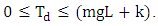 If it happens that
  becomes greater than
  then the pendulum and the beam balance rods become a rigid frame. In Autodesk Inventor-Professional (2012),
  is a product of applied damping ratio and the operating angular speed [11, 12].
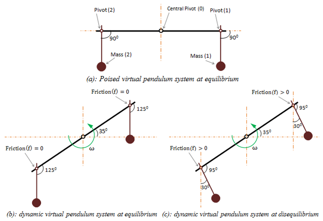 | Figure 3. Schematic diagram of the dynamic virtual pendulum system |
3. Experimental Set up
In this research there are two sets of experiments. The first set of experiments were meant to determine the torque needed at the central pivot  to drive the beam balance rod in an anticlockwise direction. The variables are; the angular speed at
  and the impeding drag force at pivot
  and
and  In summary, the power needed to drive the system as well as the power given out at pivot
  and
and  were analysed to see if they tally up to zero. The second set of experiments was meant to determine the output torque at the central pivot
  when the two pendulums are continuously displaced from their equilibriums by a driving torque (e.g. driven by an electric motor) installed at pivot
  and
and  Here the variables are; the pendulum’s angular displacement at pivot
  and
and  and the impeding drag force at pivot
  Again the main aim here was to analyse the power output at the central pivot
  against the power input at pivot
  and
and  The product of damping ratio and the angular velocity is equals to the drag force torque. Therefore to vary the output power, drag force torque needs to be varied. However, to vary the value of drag force torque the damping ratio and/or the angular velocity will have to be varied. In Autodesk Inventor-Professional (2012), damping ratio is given in the units of; Nmm s/deg. Angular velocity on the other hand is given in the units of; deg/s. [13, 14]
4. Experimental Results and Discussion
As discussed in section 3.1, there are two sets of experiments. The first set of experiments are those in section 4.1 while the second set off experiments are those in section 4.2. Moreover each set has four experiments. Therefore in total there are eight experiments in this research.
4.1. Input Power at (p0) Verses Output Power at (p1) and (p2)
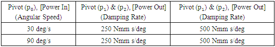
In this set of experiments the pivot  (i.e. beam balance rod) is made to rotate in an anticlockwise manner at an angular speed of 30 deg/s and 90 deg/s independently. Keeping a particular speed constant, the damping ratio at
  and
and  are varied from (250 Nmm s/deg) to (500 Nmm s/deg) independently. The layout of the experiments is as shown in table 1.
Table 1. Layout of the first set of experiments
 |
| |
|
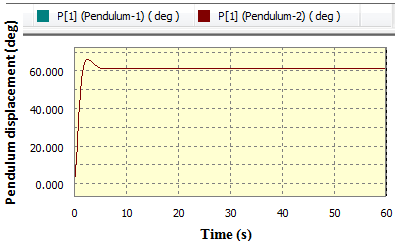
4.1.1. 30 deg/s at (p0) and 250 Nmm s/deg damping at (p1) and (p2)
Figure 4 (a) shows a graph of input and output power in watts against time. Figure 4(b) shows the graph of Pendulum’s angular displacement from its original vertical equilibrium in relation to time.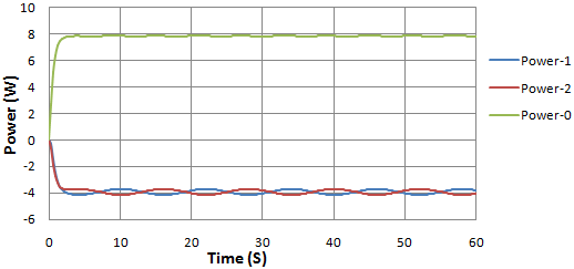 | Figure 4(a). Input and output power in watts against time |
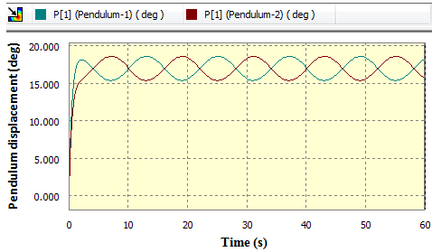 | Figure 4(b). Pendulum’s angular displacement in deg against time |
4.1.2. 30 deg/s at (p0) and 500 Nmm s/deg damping at (p1) and (p2)
In this experiment the conditions in section 4.1.1 have been kept constant and only the damping ratio at  and
and  has been increased from 250 Nmm s/deg to 500 Nmm s/deg.
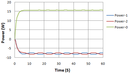 | Figure 5(a). Input and output power in watts against time |
 | Figure 5(b). Pendulum’s angular displacement in deg against time |
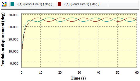
4.1.3. 90 deg/s at (p0) and 250 Nmm s/deg damping at (p1) and (p2)
The graph in figure 6 (a) show the variations in input and output power against time. On the other hand figure 6 (b) is a graph of Pendulum’s angular displacement from its original vertical equilibrium.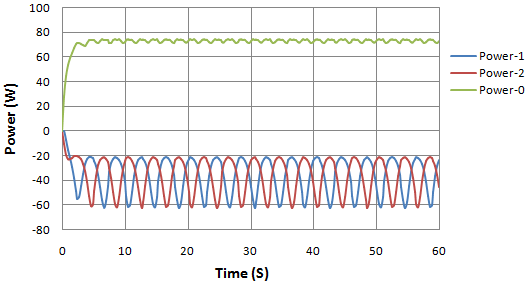 | Figure 6(a). Input and output power in watts against time |
 | Figure 6(b). Pendulum’s angular displacement in deg against time |
From graphs in section 4.1.1 to section 4.1.3 it can be noticed that the power input at pivot  is equal to the sum of the power output at pivot
  and
and  Also observed is the constant wavy nature of the pendulum’s angular displacement.
4.1.4. 90 deg/s at (p0) and 500 Nmm s/deg damping at (p1) and (p2)
In this experiment the conditions in section 4.1.3 have been kept constant and only the damping ratio at  and
and  has been increased from 250 Nmm s/deg to 500 Nmm s/deg. However the outcome of this experiment as seen in figure 7 (a) are of a capricious nature. It is noted that; in this experiment the pendulum dose not only shifts its equilibrium but makes a complete and continuous rotation round its axis as shown in figure 7 (b).
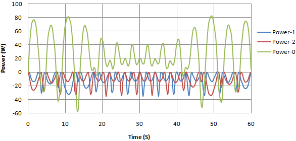 | Figure 7(a). Input and output power in watts against time |
 | Figure 7(b). Pendulum’s angular displacement in deg against time |
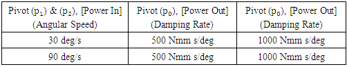
4.2. Output Power at (p0) Verses Input Power at (p1) and (p2)
For this experiments the pivot  and
and  (i.e. pendulum rod 1 and 2) was made to rotate in an anticlockwise manner at angular speed of, 30 deg/s and 90 deg/s independently. However, since the entire system was then displaced from its equilibrium, a clockwise rotation of the beam balance was induced. This therefore meant that, the pendulum rod could not make a complete absolute rotation in its on axis but rather experienced just an anticlockwise angular displacement from its original vertical equilibrium. Table 2 shows the layout of the second set of experiments.
Table 2. Layout of the second set of experiments
 |
| |
|
4.2.1. 30 deg/s at (p1) and (p2) and 500 Nmm s/deg damping at (p0)
As seen from figure 8 (a) the input power in each of the pendulums is of an undulating nature while the output power at  seems to be linear, nevertheless with low vibration.
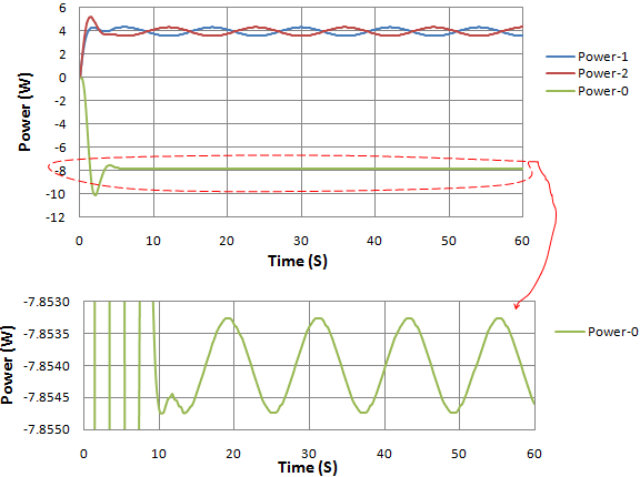 | Figure 8(a). Output and input power in watts against time |
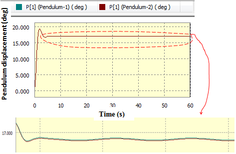 | Figure 8(b). Pendulum’s angular displacement in deg against time |
4.2.2. 30 deg/s at (p1) and (p2) and 1000 Nmm s/deg damping at (p0)
As seen in figure 9 (a) the input power in each of the two pendulums is  Consequently the output power at
  is equal to
  The new equilibrium of the two pendulums is at an angle of
  from the original vertical equilibrium as depicted in figure 9 (b).
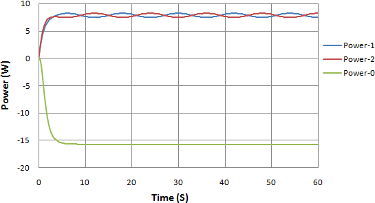 | Figure 9(a). Output and input power in watts against time |
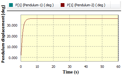 | Figure 9(b). Pendulum’s angular displacement in deg against time |
4.2.3. 90 deg/s at (p1) and (p2) and 500 Nmm s/deg damping at (p0)
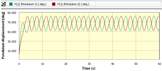
As seen in the graph in figure 10 (a) the input power adopts a crimpy nature while the output power adopts a more or less linear nature. Figure 10 (b) shows that the two pendulums are displaced to an angle of  from the original vertical equilibrium.
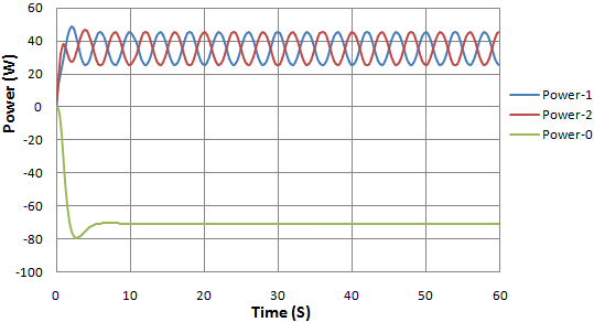 | Figure 10(a). Output and input power in watts against time |
 | Figure 10(b). Pendulum’s angular displacement in deg against time |
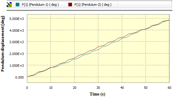
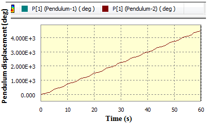
4.2.4. 90 deg/s at (p1) and (p2) and (1000 Nmm s/deg) damping at (p0)
The outcome in this experiment is similar to that in section 4.1.4. As seen in figure 11 (a) the variations in the rate of energy input and energy output is high. At some instances the pivots  and
and  which are suppose to be points of power input turn to be points for power output. Moreover the pendulums make a continuous rotation round the pivots
  and
and  as shown in figure 11 (b).
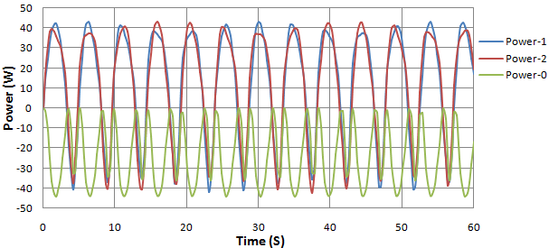 | Figure 11(a). Output and input power in watts against time |
 | Figure 11(b). Pendulum’s angular displacement in deg against time |
5. Conclusions
The aim of this paper was to present experimental outcome of a revolving virtual pendulum system. Using “Autodesk Inventor Professional” engineering software, experiments were designed to study any resultant torque within the system and there effects on energy balance. Analysis showed that, damping or friction at  and
and  shifts the equilibrium of pendulum 1 and 2 from their natural vertical position when the two pendulums are revolved on a circular orbit whose centre is
  . This in turn causes the entire system to be at disequilibrium and hence a resultant torque at pivot
  . Further the resulting torque determines the input power at pivot
  . However the output power is determined by the angular displacement of the pendulums.The wavy nature of the graph representing the pendulum’s angular displacement is attributed to the effects of “centrifugal acceleration acting radialy outwards” trying to balance out with the “gravitational acceleration acting vertically downwards”. At high angular speed and high damping ratio the system becomes patchier in its dynamism and is therefore not easily predictable.In summary it can be inferred that: presents of friction or any form of resistance at the pivot of the hanging pendulum affects the input power of revolution in a direct proportion. This means that if the sitting chair of a vertical merry go round is at a local disequilibrium, more power will be needed to revolve the entire system. However it is important to note that useful information was generated that could help when designing future systems containing a revolving hanging pendulum. Further experiments could be done involving angular speeds higher than 100 deg/s.
ACKNOWLEDGEMENTS
Special thanks go to my parents Mr. and Mrs David Kipkononden Towett for their financial and emotional support. My tribute also goes to the departments of Energy Engineering, Mechanical and Production Engineering Moi University. Finally, I cannot forget my creator and God for his absolute grace and tender mercies.
References
| [1] | Pendulums. Retrieved September 12, 2015, from http://www.sparknotes.com/testprep/books/sat2/physics/chapter8section5.rhtml Properties of Pendulum Motion. |
| [2] | Angrist, Stanley. "Perpetual Motion Machines". Scientific American. 218 (1): 115–122. Bibcode: 1968SciAm.218a.114A, 1968. |
| [3] | "Definition of perpetual motion". Oxforddictionaries.com. 2012-11-22. Retrieved 2012-11-27. |
| [4] | Ord-Hume, Arthur WJG. Perpetual motion. Adventures Unlimited Press, 2015. |
| [5] | Schaffer, Simon. "The show that never ends: perpetual motion in the early eighteenth century." The British journal for the history of science 28.2 (1995): 157-189. |
| [6] | Åström, Karl Johan, and Katsuhisa Furuta. "Swinging up a pendulum by energy control." Automatica 36.2 (2000): 287-295. |
| [7] | Nelson, R. D. and Bradish G. J. A Linear Pendulum Experiment: Effects of Operator Intention on Damping Rate (Technical Note PEAR 93003), 1933. |
| [8] | Bender, Carl M., Darryl D. Holm, and Daniel W. Hook. "Complex trajectories of a simple pendulum." Journal of Physics A: Mathematical and Theoretical 40.3 (2006): F81. |
| [9] | Jangid, R. S. "Optimum friction pendulum system for near-fault motions." Engineering Structures 27.3 (2005): 349-359. |
| [10] | Mokha, Anoop, et al. "Experimental study of friction-pendulum isolation system." Journal of Structural Engineering 117.4 (1991): 1201-1217. |
| [11] | Gembarski, Paul Christoph, Haibing Li, and Roland Lachmayer. "KBE-Modeling Techniques in Standard CAD-Systems: Case Study—Autodesk Inventor Professional." Managing Complexity. Springer, Cham, 2017. 215-233. |
| [12] | Inventor, Autodesk, and Autodesk Inventor Tooling. "Autodesk®." (2002). |
| [13] | Jaskulski, A. "Autodesk Inventor Professional." Fusion 2013pl/2013+ design methodology. PWN, Warsaw (2012). |
| [14] | Waguespack, Curtis. Mastering Autodesk Inventor 2014 and Autodesk Inventor LT 2014: Autodesk Official Press. John Wiley & Sons, 2013. |

 Abstract
 Reference
 Full-Text PDF
 Full-text HTML