Ezugwu Chinedu A. K.1, Okonkwo Ugochukwu C.2, Sinebe Jude E.3, Okokpujie Imhade P.2
1Landmark University, Omu-Aran, Nigeria
2Department of Mechanical Engineering, Nnamdi Azikiwe University, Awka, Nigeria
3Department of Mechanical Engineering, Delta State University, Oleh Campus, Nigeria
Correspondence to: Okonkwo Ugochukwu C., Department of Mechanical Engineering, Nnamdi Azikiwe University, Awka, Nigeria.
| Email: |  |
Copyright © 2016 Scientific & Academic Publishing. All Rights Reserved.
This work is licensed under the Creative Commons Attribution International License (CC BY).
http://creativecommons.org/licenses/by/4.0/

Abstract
Regenerative chatter is an instability phenomenon in machining operation that must be avoided if high accuracy and greater surface finish is to be achieved. It comes with its own consequences such as poor surface finish, low accuracy, excessive noise, tool wear and low material removal rate (MRR). In this paper, an analytical method base on first order least square approximation full-discretization method is use for the stability analysis on the plane of axial depth and radial depths of cut. A detail computational algorithm has been developed for the purpose of delineating stability lobe diagram into stable and unstable regions using mathematical models. These algorithms enabled the performance of sensitivity analysis. From the results axial depth of cut enhances the unstable region and suppresses the stable region. This means that inverse relationship exists between the axial and limiting radial depths of cut thus highlighting the need to determine the maximum value of their product for achieving maximized MRR thereby reducing the chatter in the milling process. It is also seen that the peak radial depths of cut occasioned by the lobbing effects occur at fixed spindle speeds irrespective of the axial depth of cut. Similarly, the rise in spindle speed enhances the stable region and suppresses the unstable region. This means that for us to have chatter-free milling process, parameters like axial and radial depths of cut should be carefully selected together at high machining speed. With these behaviour, one can locate the productive spindle speed at which the lobbing effects occur and depths of cut combination for the operator.
Keywords:
Delineation, Regenerative chatter, Full discretization, Stability lobs diagram, Milling
Cite this paper: Ezugwu Chinedu A. K., Okonkwo Ugochukwu C., Sinebe Jude E., Okokpujie Imhade P., Stability Analysis of Model Regenerative Chatter of Milling Process Using First Order Least Square Full Discretization Method, International Journal of Mechanics and Applications, Vol. 6 No. 3, 2016, pp. 49-62. doi: 10.5923/j.mechanics.20160603.03.
1. Introduction
Milling is an intermittent process in which shock loads are associated with both engagement and disengagement of the teeth with the workpiece [1]. Milling machine is widely used for the higher material removal rate (MRR) operating at very high speed [2]. Because of high speed, dynamic problem occurs in milling machine spindle and tool. As there is relative motion between tool and work piece, various internal and external forces rises in tool and work piece. These forces set up vibration in machine part which is in motion or in rest. Basically three types of vibration occur in machine, free vibration, forced vibration and self-excited vibration [3]. First two vibrations can be easily detected and controlled by using dampers and by other means. But, mainly chatter prediction is major task for the operator while operating at higher speed. It has a very poor surface finish which directly decreases the productivity [4]. The recent trends in manufacturing industry have an expanding requirement for enhanced characterization of cutting tools for controlling vibration and chatter amid the processing procedure [5]. The chatter is a self-excitation phenomenon happening in machine tools, in which the cutting process tends to diminish the machine structural damping resulting in an unstable condition [1]. Though chatter prediction is tough task, the area of interest in this work is to identify how the effect of regenerative chatter can be felt in pocket milling through the delineation of the stability lobs. Chatter is broadly classified in two categories: Primary chatter and secondary chatter. Primary chatter is sub classified as frictional chatter, thermo-mechanical chatter and mode-coupling chatter. Primary chatter is because of the friction between tool and work piece and it diminish with the increase in spindle speed. And secondary chatter is because of the regeneration of waviness of the surface of the work piece [6]. This chatter is called as regenerative chatter. This chatter is also known as self-excited chatter. It is very difficult to avoid regenerative chatter as it increases with the increase in spindle speed and depth of cut. Regenerative effect is a concept used to explain the sustained vibration occurring during machining as resulting from cutting force variation due to vibration induced surface waviness. Arnold first suggested regenerative effects as the potential cause of chatter and is now arguably considered the cause of detrimental type of machine tool vibration (Davies et al, 1999).Chatter is the most obscure and delicate of all problems facing the machinist [7]. The first stability analysis on regenerative chatter for the orthogonal cutting process was discovered by Tobias [8] and Tlusty [9]. They obtained stability lobe diagram (SLD) on the basis of stability analysis. It shows the boundary between stable an unstable cut. By using SLD, operator may select chatter free operations for the milling machine. A detailed discussion can be seen in many papers regarding SLD. Chatter vibration has various negative effects such as: × Poor surface quality and unacceptable accuracy,× Tool wear and tool damage,× Excessive noise,× Low material removal rate (MRR),× Low productivity rate.
2. Phenomenon of Regenerative Chatter
The milling process is most pronounced if the material removal rate is large enough while maintaining a high quality level [10]. The topmost limitation in machining productivity and part quality are the instability phenomenon that is frequently witness in cutting operations called regenerative chatter [11, 12]. The chatter vibrations of machine tool occur due to a self-excitation mechanism in the generation of chip thickness during machining operations. Due to the cutter vibrations a wavy surface is left on the surface of the workpiece by means of a tooth of cutter [13]. Then the very next tooth strikes the wavy surface and generates the new wavy surface as can be seen in the figure. 1 bellow. The phase difference between the two wavy surfaces varies the chip thickness. This increase the cutting forces of cutter. Then system becomes unstable, and chatter vibrations grow until the tool jump out of the cut which results in non-smooth surface. Thus if the chatter vibrations continue the material removal rate will be greatly affected [9].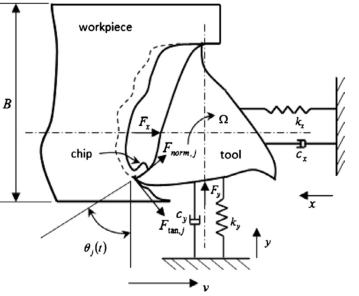 | Figure 1. Regenerative wave milling model |
3. Milling Chatter Model
Two degree of freedom milling model is the form of milling model chosen for this work more and this is because of lack of rigidity of the tool in its transverse plane causing compliance in both the feed and normal to feed directions.The free-body diagram for the tool dynamics when the motion of the tool  is considered to be a summation of feed motion and vibrations is as shown in Fig. 2.
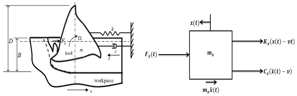 | Figure 2. (a) 1-DOF dynamic model (b) Free-body diagram of tool dynamics |
The differential equation governing the motion of the tool as seen from the free-body diagram above now becomes | (1) |
A tool-workpiece disposition is considered for the  tooth of the tool. The cutting force is considered as having normal and tangential components designated
  and
and  respectively. Axial component of cutting force is neglected because helix angle is considered zero. The
  component of cutting force for the tool thus becomes
 | (2) |
The cutting forces on  tooth are given by the non-linear law as follows
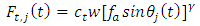 | (3a) |
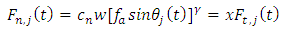 | (3b) |
The symbols  and
and  are the tangential and normal cutting coefficients which are numerically influenced by workpiece material properties and tool shape. The symbol
  stands for the number of tool teeth. Where
  is the depth of cut,
  is the ratio of
  ,
,  is the actual feed given as
 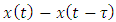 which is the difference between present and one period delayed position of tool and
  is an exponent that is usually less than one, having a value of ¾ for the three-quarter rule. The instantaneous angular position of
  tooth
tooth  is given as
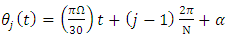 | (4) |
where  is the spindle speed in rpm and
  is the initial angular position of the tooth. The screen function
  has values of either unity or nullity depending on whether the tool is cutting or not. Given start and end angles of cut
  respectively,
  becomes
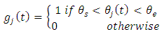 | (5) |
The mathematical form for  is given as
  | (6) |
For up milling  are expressed in terms of radial depth of cut b [22]
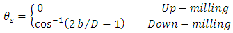 | (7a) |
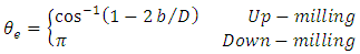 | (7b) |
Figure 3 below is a 2 DOF depiction of an end-milling tool, with the stiffness and damping elements oriented in the  plane (horizontal plane). The modal parameters
  and
and  are for
  vibration while
  and
and  are for
  vibration
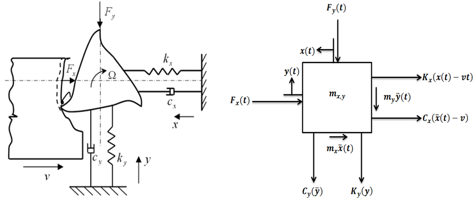 | Figure 3. (a) 2-DOF tool dynamics (b) Free-body diagram of toll dynamics |
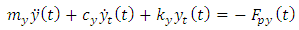
The governing equation of motion now becomes | (8a) |
 | (8b) |
The  and
and  component of the cutting force on the tool are
 | (9a) |
 | (9b) |
The actual feed rate  of
of  tooth at angular position
  is given as
 | (10) |
where  .The quantity
  and
and  are perturbations in the
  and
and  directions respectively.The linearized Taylor series expansion of
  about
about  then reads
 | (11) |
When  and
and  are considered to be zero in equations (11), (3a-3b) and (9a- 9b) above, we will form equations (12a) and (12b) from equations (8a) and (8b)
 | (12a) |
 | (12b) |
Where | (13a) |
 | (13b) |
The periodic forces  and
and  respectively drives the two orthogonal
  periodic tool responses
  and
and  .Putting equations (12a-12b) into equation (8a-8b) and simplifying give
  | (14a) |
 | (14b) |
In the light of specific periodic cutting force variations, we have as  | (15a) |
 | (15b) |
 | (15c) |
 | (15d) |
Equations (14a) and (14b) are put in matrix form gives  | (16) |
Where  is the vector of chatter vibration in the two orthogonal directions of
  and
and  , the mass M, damping C and stiffness K matrices are respectively given as
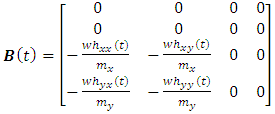
 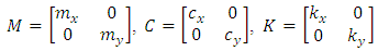 | (17) |
The forcing function in equation (17)  contains a time-periodic function
  that results from rotational motion of the milling teeth
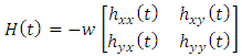 | (18) |
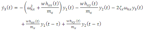
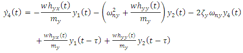
By pre-multiplying equation (16) with the inverse of the mass matrix, the modal form of the governing model upon little re-arrangement becomes | (19) |
The expanded form of equation (19) when each of the matrix operations  and
and  are carried out reads
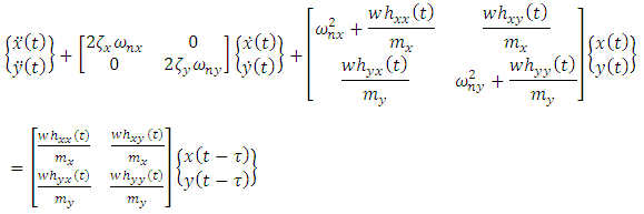 | (20) |
Equation (20) is the model for milling chatter whose stability behaviour is of interest in this work.
4. Progress in Stability Analysis of Milling
Stability analysis of milling process is normally carried out on either the state space form or non-state space form of the governing model. Most stability analysis carried out on milling process using the methods of semi-discretization [14, 5], temporal finite element analysis [16] and the full-discretization method [17, 18] are formulated on the state space form of the governing model while stability analysis based on the methods of Zero order approximation or multi-frequency solution can be formulated on the non-state space version of the governing model. Considering the governing model (equation (20)), four state variables can be identified;  . The state variables are then designated as follows;
  and
and  . For better understanding of the process of state space transformation of equation (20), two constituent equations are written out as
 | (21a) |
 | (21b) |
In light of the identified state variables, equation (21a-21b) can be re-written as | (22a) |
 | (22b) |
 | (22c) |
 | (22d) |
It is seen that equation (22a-22d) is the four-dimensional state space form written in compact form as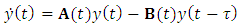 | (23) |
Where  (the superscript “T” means transposition)
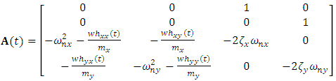 | (24) |
 | (25) |
Equation (23) is then re-arranged by splitting matrix  into
into  and a constant matrix
  so that the governing model can conform with the full-discretization method such that equation (23) becomes
  | (26) |
where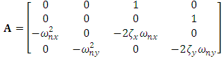 | (27) |
The procedure which involves discretizing the system’s period and interpolating or approximating the solution in the discrete intervals is adopted for this work. The full-discretization method is the choice of stability analysis in this work because it has been proven to save more computational time than the semi-discretization method. This is due to the introduction of interpolation polynomials in the integration scheme of full-discretization method which upon solving produces a discrete map that is used for stability analysis. The full-discretization method is heavily based on discretization. The discretization and solution schemes are summarized from the work [18] to involve dividing the period of the governing full-discretization model (equation (26))  into
into  equal discrete time intervals
  where
where  and
and  . Equation (26) is then handled as the governing model in the general discrete interval
  . The solution in the discrete interval
  arises from definite integration between the limits
  and
and  to become
 | (28) |
What differentiates various full-discretization methods is the manner of proceeding from equation (28). The original full-discretization method [17] approximated the milling solution or motion  with the tool of linear interpolation theory. Other subsequent full-discretization methods which are seen in the reference list of the work [18] are also based on interpolation theory of various orders and kinds (i.e, Lagrange, Newton and Hermite interpolation theories). The work [18] has introduced full-discretization methods for which the milling motion
  is approximated with least squares theory to yield considerable savings in computational time. The first-order least squares approximation of the state terms
  and
and  is as followsThe first order least squares approximation of the state term
  is seen as
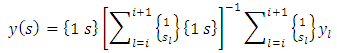 | (29) |
It should be noted that  and
and  in the summation signs of equation (29) corresponding to terms at
  and
and  . This is re-written as
 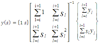 | (30) |
Equation (30) is further re-written as 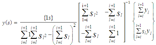 | (31) |
The above equation is multiply to give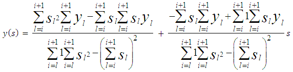 | (32) |
By carrying out the summation in equation (32) and simplifying it gives equation (33a) | (33a) |
With the substitution of  and
and  , Equation (33a) is put in the form
 | (33b) |
In the same way as above, the delay state  and periodic coefficient matrix
  will also give as
  | (34) |
 | (35) |
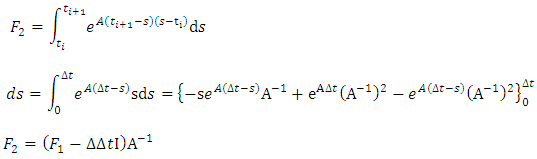
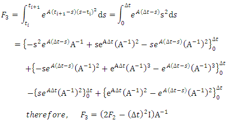
Equations (33a), (34) and (35) are inserted into equation (28) to give 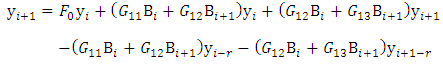 | (36) |
Where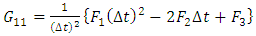 | (36a) |
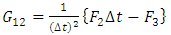 | (36b) |
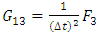 | (36c) |
 | (37a) |
and 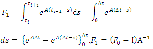 | (37b) |
 | (37c) |
 | (37d) |
The equation (36) is re-arranged to become | (38) |
Where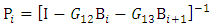 | (39) |
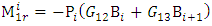
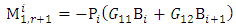
The local discrete map derived from equation (38) is given by [15] 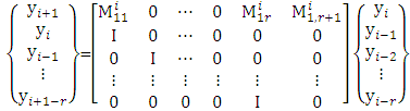 | (40) |
where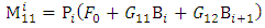 | (41a) |
 | (41b) |
 | (41c) |
The stability matrix for the system becomes [15]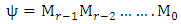 | (42) |
Where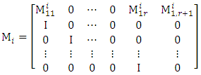 | (43) |
The aim of the afore-conducted mathematical analysis is derivation of the stability matrix  . Utilizing the matrices in equations (36a-36c), (37a-37d), (39), (41a-41c) and (43) in the stability matrix of equation (42) is all that is needed for stability characterization of the system. This obviates the need to go through the mathematical rigorous of this chapter by any reader interested only in the stability matrix and stability computation. The nature of eigen-values of the stability matrix is the criterion for stability characterization of milling process. Asymptotic stability requires all the
  eigen-values of the stability matrix
  to exist within the unit circle centred at the origin of the complex plane [18]. Stability boundary of milling process is then a curve that joins the critical parameter combinations at which maximum-magnitude eigen-values of
  lie on the circumference of the unit circle [18]. Milling stability lobes are computed with a value of
  that is big enough to guarantee benchmark accuracy [19]. Computations in literature are normally computed on
  by
by  grid on the plane of spindle speed and axial depth of cut. Computations in this work will include computing on
  by
by  grid on the plane of spindle speed and radial depth of cut.
5. Algorithms for Computation of Stability Limits of Milling
Delineation of milling process into stable or unstable occasioned by chatter can only have a real, physical or numerical reality when the constant parameters (which include tool, prescription and cutting parameters) are known numerically. The knowledge of tool and cutting parameters can stem from either pure experimental analysis or hybrid of experimental and numerical/theoretical analysis [20, 22]. Stability limits of the milling process can be computed by calculation, sorting and mapping of the eigen-values of the stability matrix  given in equation (42). As stated earlier, stability limit of milling process is a curve that joins the critical parameter combinations at which maximum-magnitude eigen-values of
  lie on the circumference of the unit circle. This means that stability limit is arrived at when all parameters combinations at which eigen-values of unit magnitude are calculated, sorted out and connected by a curve. Computations of milling stability limit in literature normally give axial depth of cut as a function of spindle speed at a given value of radial depth of cut. Numerical computations of milling stability limit in the next section will include giving radial depth of cut as a function of spindle speed at a given value of axial depth of cut and giving radial depth of cut as a function of axial depth of cut at a given value of spindle speed. The procedures for these computations are spelt out in the following algorithms.Algorithm 1The algorithm for computation of stability limits of milling giving axial depth of cut as a function of spindle speed at a fixed value of radial depth of cut which is based on the analytical development in previous sections is as follows;1. Provide the values of tool and cutting parameters given. Also provide the approximation parameter r, radial immersion
  , the step and number of steps of computation for both axial depth of cut and spindle speed.2. Compute the time-invariant matrix
  and its inverse.3. Chose the first step of spindle speed and compute the discrete delay or period
  , the discrete time step range
  , the
, the  and
and  matrices.4. Chose the first step of axial depth of cut with spindle speed fixed as chosen in 3 and form discrete time intervals
  where
where  and
and 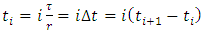 . At the extremities of the first discrete time interval
  compute
  and use the result to form the matrices
  . Use the G matrices together with the matrices
  and
and  to form the matrix
  . Then form the matrices
  from the G matrices
  . Making use of the matrices
  form the matrix
  .5. Carry out the operation in algorithm step 4
  times at the remaining steps
  and use result of all the steps to form the stability matrix
  . Compute the eigen-values of
  and chose the eigen-value with maximum magnitude.6. Repeat steps 4 and 5 for the remaining steps of axial depth of cut.7. Repeat steps 3-6 for the remaining steps of spindle speed.8. Connect the parameter combinations of spindle speed and axial depth of cut at which maximum magnitude of eigen-values is unity to form the stability limit.Algorithm 2On the other hand the algorithm for computation of stability limits of milling that presents radial depth of cut (or radial immersion) as a function of spindle speed at a fixed value of axial depth of cut is as follows;1. Provide the values of tool and cutting parameters given. Also provide the approximation parameter r, axial depth of cut, the step and number of steps of computation for both radial depth of cut and spindle speed.2. Compute the time-invariant matrix A and its inverse.3. Chose the first step of spindle speed and compute the discrete delay or period
  , the discrete time step range
  , the F and G matrices.4. Chose the first step of radial depth of cut with spindle speed fixed as chosen in 3 and form discrete time intervals
  where
where  and
and  . At the extremities of the first discrete time interval
  compute
  and utilize it together with the chosen radial depth of cut to compute
  then compute
  and use the results to form the matrices
  and
and  . Use the G matrices together with the matrices
  and
and  to form the matrix
 . Then form the matrices
  ,
,  and
and  from the G matrices,
  ,
,  and
and  and
and  . Making use of the matrices
  form the matrix
  . 5. Carry out the operation in the algorithm step4
  times at the remaining steps
  and use result of all the steps to form the stability matrix
  . Compute the eigen-values of
  and chose the eigen-value with maximum magnitude.6. Repeat steps 4 and 5 for the remaining steps of radial depth of cut.7. Repeat steps 3-6 for the remaining steps of spindle speed.8. Connect the parameter combinations of spindle speed and radial depth of cut at which maximum magnitude of eigen-values is unity to form the stability limit.Algorithm 3Stability limits of milling on the plane of axial depth of cut and radial depth of cut at fixed spindle speed is generated by following the algorithm that follows;1. Provide the values of tool and cutting parameters. Also provide the approximation parameter r, the fixed spindle speed, the step and number of steps of computation for both axial and radial depths of cut.2. Compute the time-invariant matrix A and its inverse, the discrete delay or period
  , the discrete time step range
  and the F and G matrices.3. Chose the first step of axial depth of cut then chose the first step of radial depth of cut. Form discrete time intervals
  where
where  and
and  . At the extremities of the first discrete time interval
  compute
  and utilize it together with the chosen radial depth of cut to compute
  then compute
  and use the results to form the matrices
  and
and  . Use the G matrices together with the matrices
  and
and  to form the matrix
  . Then form the matrices
 from the G matrices,
  . Making use of the matrices
  form the matrix
  . 4. With the axial depth of cut fixed at value in step4 carry out the operation in the algorithm step 4
  times at the remaining steps
  and use result of all the steps to form the stability matrix
  . Compute the eigen-values of
  and chose the eigen-value with maximum magnitude.5. Repeat steps 3 and 4 for the remaining steps of radial depth of cut.6. Repeat steps 3-6 for the remaining steps of axial depth of cut.7. Connect the parameter combinations of axial and radial depths of cut at which maximum magnitude of eigen-values are unity to form the stability limit.Each of the three presented algorithms above will be utilized to generate stability limits that will be jointly used to delineate the stability lobs diagram [22].
6. Results and Discussion
Simulation of Stability Limits of MillingStability limits from algorithms 1 and 2 are the ones that combine to give the spindle speed of productive depth of cut. Such spindle speeds, when ascertained are utilized in the algorithm 3 for generating of stability limit that allows selection of the maximum product  at which MRR may be maximized. The graphs of all the aforementioned algorithms are mapped out with MATLAB for stability milling process on three different plane of parameter space of the prescription parameters for comparative analysis. Numerical values of parameters to be use in the stability analysis is borrowed from Weck et al as cited in [23] and are presented thus:


 . Where subscripts
  represents independent coordinates in
  -directions respectively,
  is the natural frequency, k is the stiffness,
  is the damping ratio, m is the modal mass, N is the number of teeth on the milling tool,
  is the start angle of cut while
  represents tangential and normal cutting coefficients respectively.Using parameters above and following algorithm 1 gives stability limits of milling on the plane of spindle speed and axial depth of cut at selected fixed radial immersions seen in figure 4 bellow.
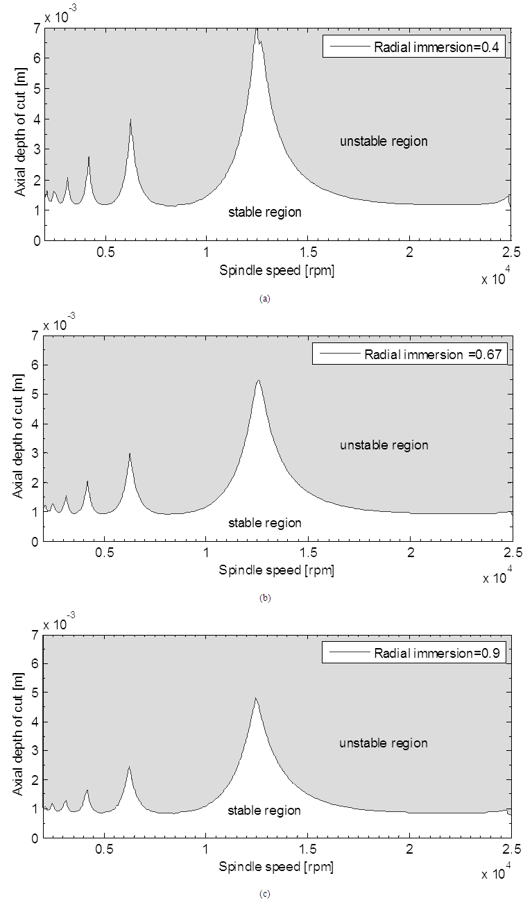 | Figure 4. Stability Limits of Milling on the Plane of Spindle Speed and Axial Depth of Cut at Selected Fixed Radial Immersions |
It can be deduced from above figure that rise in radial immersion enhances the unstable region and suppresses the stable region which is as a result of chatter. This means that there is some kind of inverse relationship between the axial and radial depths of cut highlighting the need to determine the maximum value of their product for achieving maximized MRR thereby reducing the chatter in the milling process. The other important observation is that the peak axial depths of cut occasioned by the lobbing effects occur as fixed spindle speeds irrespective of value of the radial immersion. This observation is very useful for implementation of algorithm 3. It must be noted that figure 5b is validated by the figure generated with identical set of parameters in [24] meaning that algorithm 1 which is based on theoretical development in this work provides reliable stability limit of milling process.When the same parameters are used in algorithm 2, it gives stability limits of milling on the plane of spindle speed and radial depth of cut at selected fixed axial depth of cut seen in Figure 5.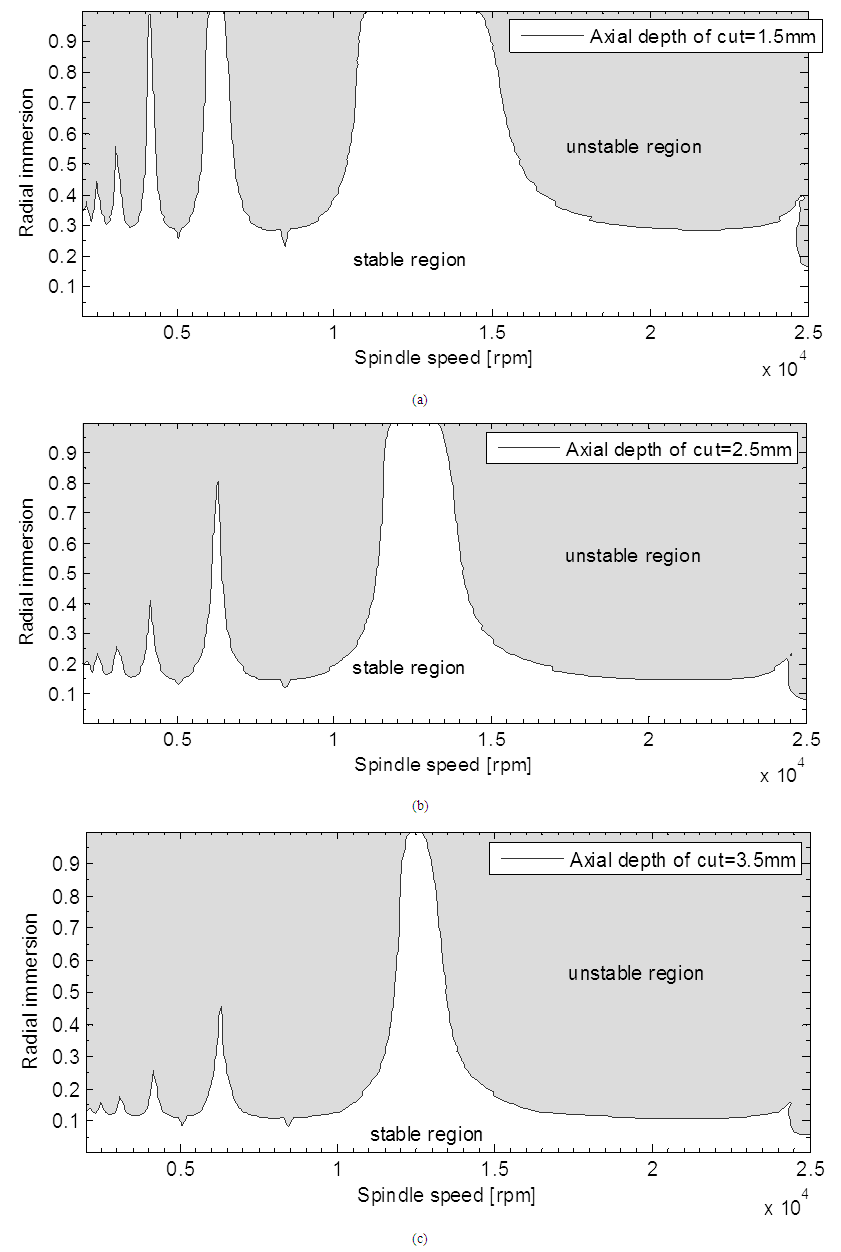 | Figure 5. Stability limits of milling on the plane of spindle speed and radial depth of cut at selected fixed axial depths of cut |
Figure 5 shares similar behaviour with Figure 4. It is seen in Figure 5 that rise in axial depth of cut enhances the unstable region and suppresses the stable region. This means that inverse relationship exists between the axial and limiting radial depths of cut thus highlighting the need to determine the maximum value of their product for achieving maximized MRR thereby reducing the chatter in the milling process. It is also seen that the peak radial depths of cut occasioned by the lobbing effects occur at fixed spindle speeds that are same as in figure 4 irrespective of value of the axial depth of cut. This observation which is consistent with figures 4 and 5 means that implementing algorithm 3 at any of such productive spindle speeds will generate the most productive stability limits of milling on the plane of axial depth of cut and radial depth of cut. It must be noted that figure 5a is validated by the figure generated with identical set of parameters in [24] meaning that algorithm 2 which is based on theoretical development in previous sections of this work provides reliable stability limit of milling process.Using the same parameters above in algorithm 3, stability limits of milling on the plane of axial depth of cut and radial depth of cut at the selected productive spindle speeds 4208, 6270, 12600 were generated as seen in Figure 6.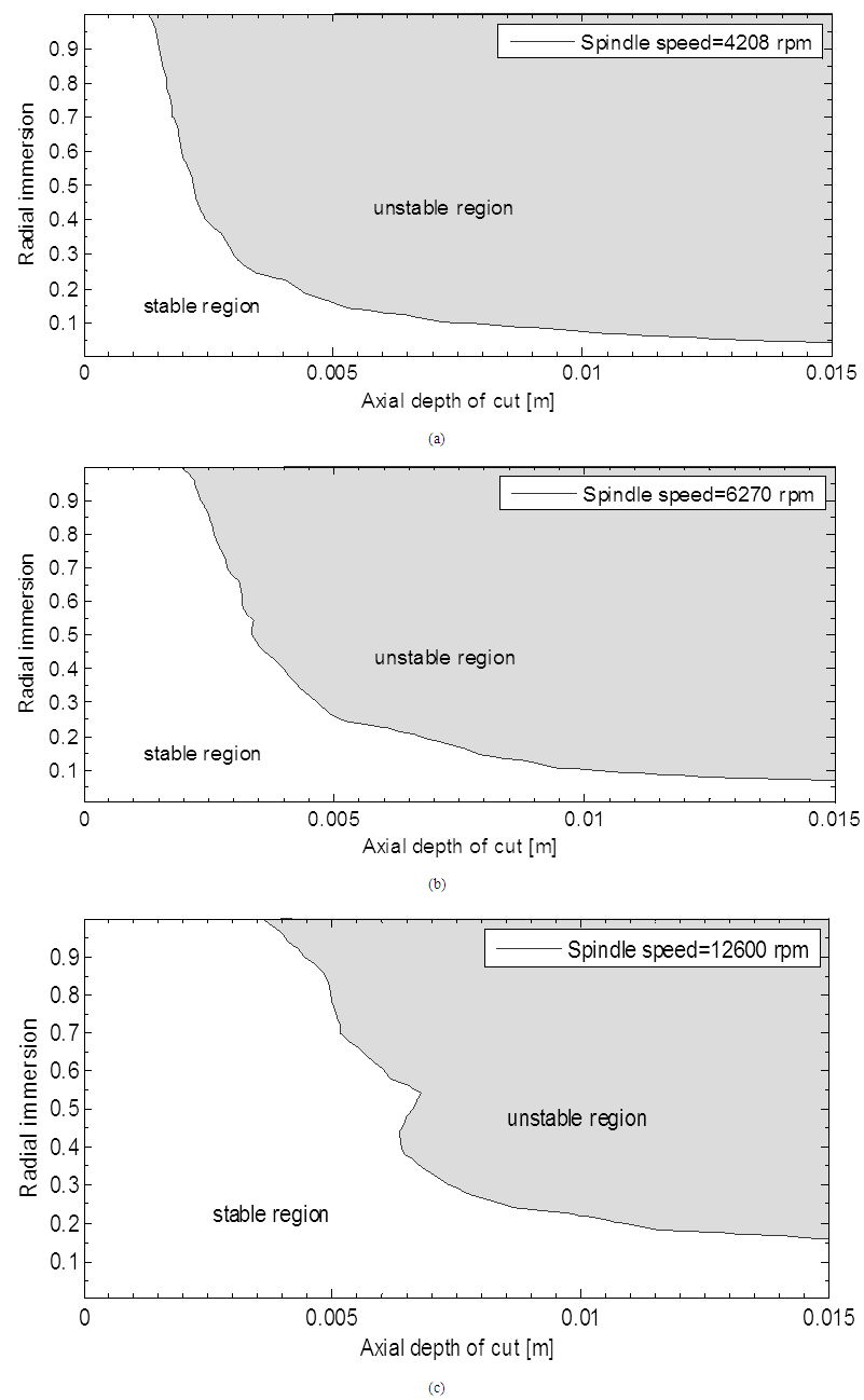 | Figure 6. Stability limits of milling on the plane of axial depth of cut and radial depth of cut at selected productive spindle speeds |
The inverse relationship between limiting axial depth of cut and limiting radial depth of cut suggested by figures 4 and 5 is actually true looking at figure 6. It is seen in figure 6 that rise in spindle speed enhances the stable region and suppresses the unstable region. This means that for us to have chatter-free milling process, parameters like axial and radial depths of cut should be carefully selected together at high machining speed. It must be noted that figure 6c agrees closely with the figure generated with identical set of parameters in [24] meaning that algorithm 3 for the first order least squares approximated map of the work [18] provides reliable stability limit of milling process on the plane of depths of cut.
7. Conclusions
Regenerative chatter poses serious challenge to machine operator this days in achieving high accuracy and acceptable surface finish. Various methods are available for the control of chatter. Some are analytical, semi-analytical while others are experimental. Some of the results of this work can be identified to be new in the field optimal machining. The work lays the foundation for use of the least squares approximated full-discretization method in stability analysis on the plane of axial depth of cut and radial depth of cut using analytical method. A detailed computational algorithm was presented for the purpose of delineating stability lobe diagram into stable and unstable regions. The stability lobe diagram if well understood, will be a guide to operators in selecting a chatter free spindle speed and depths of cut knowing that there are some spindle speed that are not productive and also the proper combination of the depths of cut so as to boost surface finish and greater accuracy.
References
| [1] | Osueke C.O, Ezugwu C.A.K, Adeoye A.O (2015) Dynamic approach to optimization of material removal rate through programmed optimal choice of milling process parameters, part 1: validation of result with CNC simulation. International Journal of innovative research in Advanced Engineering, 2(5), 118-129. |
| [2] | Okokpujie Imhade P., Okonkwo Ugochukwu C., Okwudibe Chinenye D. (2015) Cutting parameters effects on surface roughness during end milling of aluminium 6061 alloy under dry machining operation. International Journal of Science and Research, 4(7), 2030-2036. |
| [3] | Altintas, Y., "Manufacturing Automation: Metal Cutting Mechanics, Machine Tool Vibrations, and CNC Design", 1st ed., Ed. Cambridge University Press, NY, USA, 2000. |
| [4] | Okokpujie Imhade P., Okonkwo Ugochukwu C. (2015). Effects of cutting parameters on surface roughness during end Milling of aluminium under minimum quantity lubrication (MQL). International Journal of Science and Research, 4(5), 2937-2942. |
| [5] | Tobias, S.A. (1965). Machine Tool Vibration. Blackie and Sons Ltd, 340-364. |
| [6] | Tlusty, J. and Ismail, F. (1981). Basic Nonlinearity in Machining Chatter. Annals of the CIRP, 30:21–25. |
| [7] | F. W. Taylor, “On the art of cutting metals”, Transactions of the American Society of Mechanical Engineers, pp. 31–35, 1907. |
| [8] | S.A. Tobias, Vibraciones en Maquinas-Herramientas, URMO, Spain, 1961. |
| [9] | J. Tlusty, M. Polacek, “The stability of machine tools against self-excited vibrations in machining”, International Research in Production Engineering, pp.465–474. 1963. |
| [10] | Ozoegwu C.G. & Ezugwu C. (2015). Minimizing pocketing time by selecting most optimized chronology of tool passes. International journal of advanced manufacturing technology, 79(1-4). |
| [11] | Budak, E., & Altintas, Y. (1994). Peripheral millingconditions for improved dimensional accuracy. Int. J. Mach. Tools Manufact. 34 (7) 907–918. |
| [12] | Quintana, G. and Ciurana, J. (2011). Chatter in machining processes: a review, International Journal of Machine Tools and Manufacture. International Journal of Machine tools and manufacture, 51 (5) 363–376. |
| [13] | Budak, E., and Altintas, Y. (1998). Analytical Prediction of Chatter Stability in Milling - Part I: General Formulation, Part II: Application To Common Milling Systems. Trans. ASME Journal of Dynamic Systems, Measurement and Control, 20:22–36. |
| [14] | Hashimoto, M., Marui, E., and Kato, S. (1996). Experimental research on cutting force variation during regenerative chatter vibration in a plain milling operation. International Journal of Machine Tools and Manufacture, 36 (10) 1073–1092. |
| [15] | Sridhar R, Hohn RE and Long GW. (1968). General Formulation of the Milling Process Equation, ASME J. of Eng. for Ind, 90: 317-324. |
| [16] | Ozoegwu, C. G., Omenyi, S. N., Ofochebe, S. M., and Achebe, C. H. (2013) Comparing up and Down Milling Modes of End-Milling Using Temporal Finite Element Analysis, Applied Mathematics 3(1) 1-11. |
| [17] | Ding Y, Zhu LM, Zhang XJ, Ding H. (2010). A full-discretization method for prediction of milling stability. International Journal of Machine Tools and Manufacture, 50:502–509. |
| [18] | Ozoegwu, C.G. (2014). Least squares approximated stability boundaries of milling process, International Journal of Machine Tools and Manufacture, 79, 24–30. |
| [19] | Altintas, Y., and Budak, E. (1995). Analytical Prediction of Stability Lobes in Milling. Annals of the CIRP, 44(1): 357–362. |
| [20] | Okonkwo U.C, Osueke C.O, Ezugwu C.A.K (2015) Minimizing machining time in pocket milling based on optimal combination of the three basic prescription parameters. International Research Journal of Innovative Engineering, 1(4), pp. 12-34. |
| [21] | Sridhar, R., Hohn, R.E., and Long, G.W. (1968). A Stability Algorithm for the General Milling Process. Trans. ASME Journal of Engineering for Industry, 90:330–334. |
| [22] | Ezugwu, C.A.K (2015). Minimizing Pocketing Time by Programmed Optimal Choice of Stable Milling Process Parameters: Master of Engineering Thesis, Nnamdi Azikiwe University, Awka, PP. 42- 46. |
| [23] | Tekeli, A. and E. Budak, Maximization of chatter-free material removal rate in end milling using analytical methods, Machining Science and Technology, 9:147–167. |
| [24] | Meritt, H. E. (1965). Theory of self-excited machine–tool chatter. Transactions of the ASME Journal of Engineering for Industry, 87, 447–454. |

 Abstract
 Reference
 Full-Text PDF
 Full-text HTML