1. Introduction

Several experimental and theoretical models have been studied the electromagnetic transients. In early 1969, T.T. Wu [1] stated: “It is worth emphasizing that our knowledge about the transient response of the antennas is very meager indeed. Any progress in this rather neglected field is certainly going to be of a tremendous value”. Now, the literature on this subject is vast. Some of these studies are motivated by the desire to provide adequate protection of electronic equipment in a strong electromagnetic pulse (EMP) (Vance [2]). Other studies have been applied to the probing of the fields in geological media (Wait [3]), determination of the current in a lightning return stroke (Uman and Lain [4]), the detection of nuclear bursts (Johler [5]), and the discrimination of a radar scatterer (Moffatt and Mains [6]).

In this paper will study the problem of the transient electromagnetic field of an electric line source on a two layered conducting earth. Furthermore, we will focus on the effects caused by the presence of the earth’s surface. A classical work in this area is that of Van der Pol [7] for the transient field over a non-conducting earth generated by a vertical dipole source situated in the interface between the air and the earth. The transient solution of an elevated dipole was also obtained by Van der Pol and Levelt [8] and Bremmer [9]. Wait [10, 11] and Novikov [12] studied the transient response of a vertical dipole with a step or ramp function current source over a finitely conducting earth. Since the Sommerfeld-Norton ground wave expansion is employed, which is valid for a distance large enough compared with the free space wavelength, their results are expected to be accurate mainly in the very early time portion of the response. Approximate expression for the transient field at later observation times was found by Chang [13] and Wait [14] under the assumption that the dissipative half-space can be replaced by an impedance surface.

However, an attractive alternative is furnished by De Hoop [15] modificationn of Cagniard’s technique that found wide applications in the theory of seismic waves in Cagniard [16] and [17]. Also, few electromagnetic problems have been investigated along these lines (De Hoop and Frankena [18] and Langenberg [19]). Kooij [20] and [21] studied the transient electromagnetic field of a pulsed vertical magnetic dipole above a conducting earth, and of an electric line source above a plane drude model plasmatic half-space, these showed that it is possible to arrive to a representation for the field in the transform domain that allows the application of the Cagniard-De Hoop method.

Kuester [22] investigated the transient reflected field of a pulsed line source over a conducting half-space. Bishay and Sami [23] expressed, in an analytical form the transient field in the time domain of a thin circular loop antenna on a two-layered conducting earth model.

Sami [24] calculated the influence of a magnetically permeable surface layer on transient electromagnetic field of a vertical magnetic dipole on a two-layer conducting earth.

The aim of this paper is to drive a representation for the field in the transform domain that allows the application of the Cagniard-De Hoop method to obtain the transient reflected field in the form of a single finite integral. Of particular interest is the physical insight provided by the Cagniard-De Hoop method at each point in the configuration, the transient field is decomposed exactly into physical meaningful parts. Numerical results will be represented graphically for the electric field anywhere on a two layer earth for different values of the earth`s conductivity and permittivity.

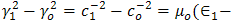
2. Description of the Configuration

We consider the electromagnetic field in the upper half space of two homogeneous, isotropic, semi-infinite media. To specify the position in the configuration, we employ the ؤartesian coordinates (x, y, z) with origin O and three mutually perpendicular base vectors (i, j, k) of unit length each. The upper medium occupies the half space 0 ≤ z < ∞, whereas the lower medium occupies the half space -∞ < z < 0, as Figure 1. The time coordinate is denoted by t, with tR. The electromagnetic properties are characterized by their permittivity , permeability , and the electrical conductivity . The media are modeled according to the classical Maxwell model with constant permittivity, permeability and conductivity. For the upper medium we have, , and . For the lower medium, we have , and . An electric current line source starts to radiate at the instant t = 0, at the earth's surface.

3. Method of the Solution

The electromagnetic field in the configuration is described in terms of the electric field strength E and the magnetic field strength H. the action of the source is characterized by specifying the volume density of its electric current J. In any domain where the field quantities are continuously differentiable, they satisfy the following electromagnetic field equations:

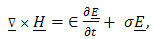(1)

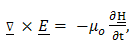(2)

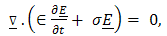(3)

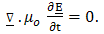(4)

There are three cases as:

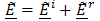
1 – Incident field , is the field that source world generate if no boundary were present.

2 – The reflected field is the difference between the total field in region0 ≤ Z < ∞ and the incident field.

3 – The transmitted field which is the field in the region across the interface of the two media, the boundary conditions below hold,

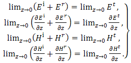(5)

Further, the primary field is the field generated by the source, should travel away from the source, and the secondary field is the field generated by the secondary sources at the inter face, should travel away from the interface (radiation condition). In media of the type under consideration, electromagnetic waves travel at the speed

(6)

To carry out our analysis, we cast the field representations in a particular from that is characteristic of the Cagniard– De Hoop method. first, we subject the field quantities to a one – sided Laplace transformation with respect to time , where the relevant transform variable (S) is taken to be real and positive the Laplace transform of quantity with respect to time by a circumflex over the relevant symbol , we have

(7)

The Fourier transformation with respect to x according to

(8)

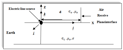Figure 1. Geometry of the problem

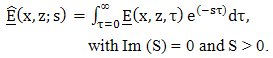
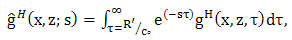
The inverse Fourier transformation,

(9)

in which ⨕ denotes the imaginary axis. Once a suitable expression for has been determined, the representation (9) is used to arrive at an expression for . This is accomplished by a specific scheme of transformations in the complex (∝) plane followed by an application of the uniqueness theorem of the one – sided Laplace transform (7).

4. Incident and Reflected Field Representations

We take into account the two – dimensionality of the problem. To this end, we decompose each vectorial quantity in to a component that is parallel to the line source, this component is denoted by the subscript and a component in the plane perpendicular to it, this component is denoted by the subscript . 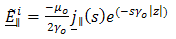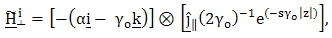Taking into account that and , we can rewrite the electromagnetic field equations (1)-(4) in a from where only an E- polarized field is generated for which and . In this section, we determine the representation of the type (9) for the incident and reflected field. The incident electromagnetic field satisfies Maxwell's equations (1)-(4) with and . For the localized line source of Figure 1, we have

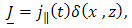(10)

Applying the transformations (7) and (8), we can get the E-polarized filed as

(11)

and

(12)

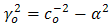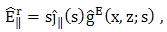
in which , when Re , and is the Dirac-delta function.

Similarly, for the reflected field, we obtain the generated E-polarized field as

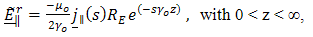(14)

and

(15)

where denotes the electric field reflection Factor for E – polarized waves. Applying the boundary condition (5), we obtain

(16)

where is given by

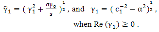(17)

5. Integral Representation of the Reflection Factor

In this section, the reflection factor R_E is rewritten in the form of an integral representation such that the Cagniard-De Hoop technique can be applied. First, we multiply both the numerator and the denominator of R_E with , then

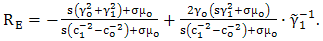(18)

The factor can be written as

(19)

where

(20)

The representation (20) can be recognized as the Laplace transform [25]

(21)

In equation (21), I_o and I₁ denote the modified Bessel functions of order zero and one, respectively. The technique of rewriting the reflection coefficient R_E as a Laplace integral is a key step that is also the basis of the exact image theory developed by Lindell and Alanen [26] and Nikoskinen and Lindell [27]. Substitution from equation (21) in equation (18) and using the fact that we obtain

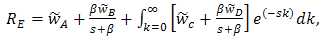(22)

where

(23)

(24)

(25)

(26)

and

(27)

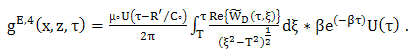
6. Time Domain Field Expressions

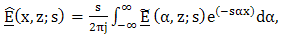
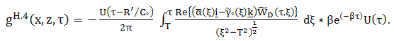
By applying the inverse Fourier transformation (9) with respect tox to equation (14) and (15) together with equation (24–29), we obtain the corresponding expressions, which are of the form

(28)

(29)

where

(30)

and

(31)

In the next step it is shown that the integrals at the right – hand side of (30) and (31) can be transformed by using (8) for Laplace transform into

(32)

and

(33)

where

(34)

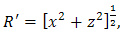
the only real values of occur in the integration and where is the distance from the image of the electric line source to the point of observation. Now, we observe that is the Laplace transform. Of a function of time that vanishes when and equal when , for the fields and , hence, we get

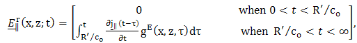(35)

(36)

where

7. Cagniard – De Hoop Technique

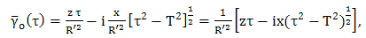
In this section, we will apply the cagniard – De Hoop technique in order to find an expression for and . In view of subsequent deformations of the path of integration, we take and not only on the imaginary axis but everywhere in the complex plane this implies that branch cuts are introduced along . Now, the path of integration in the complex plane is deformed in a cagniard – De Hoop contour defined through,

(37)

(38)

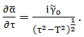
the contour is a branch of a hyperbola. let denote its parametric representation in the upper half of the complex α plan (i.e., {α∈⨕│-∞ together with its complex conjugate . By solving (37), we obtain

(39)

Along the contour, we further have

(40)

and

(41)

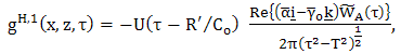
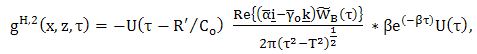
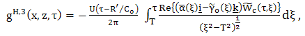
Taking into account the symmetry of the contour with respect to the real axis and reversing the orders of integration in order to apply the uniqueness argument of equation (32) – (36), we obtain,

(42)

Where

(43)

(44)

(45)

and

(46)

Similarly, we can set by using equation (32) as

(47)

where

(48)

(49)

(50)

and

(51)

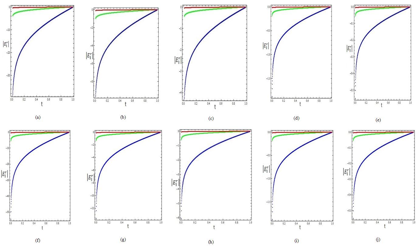Figure 2. [(a-e)and 2(f-j)] represent the normalized reflected electric field at the distance d=1m. and d=10m., where the permittivity = 2,5,10, 30 and 100, respectively. Thered, green, blue curves corresponding to the values of the conductivity , respectively

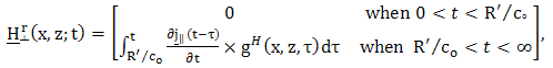
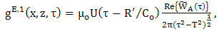
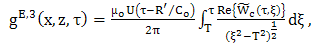
In (43) – (51) the function U denotes the Heaviside unit step function and the * symbol stands for the convolution operation with respect to . Further, we have that and . Expressions (42) and (35) form the desired closed-form expression for the space-time reflected electric field and expressions (47) and (36) form the desired closed-form expression for the space-time reflected magnetic field. Further, it is easily verified in the expression (42) and (47), together with (43) - (51), that the terms and vanish if . 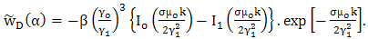In the final space-time expression of the reflected field, the convolution of the excitation function and the exponential function in (44), (46), (49), and (51) can be carried out analytically for various types of sources.

The current in the electric line source is defined by: .

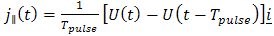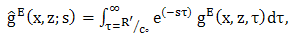
In which U (t) is the Heaviside's unit step function, is the pulse duration and . The convolution of the source function and the exponential function in (45), (47), (50) and (52) is carried out analytically. If , where denotes the numerical time discretization step, we can approximate the function by a Dirac delta function, which simplifies the expression for g^E(x, t).

8. Numerical Results and Discussion

The transient electromagnetic field due to electric line source on a two-layer conducting earth can be expressed in analytical form. The normalized reflected fields have been calculated for different values of conductivity, and ratio of permittivity , at the two distance pointe (d = 1m and 10m) of observation and excitation.

The results represented graphically and illustrated by Figure 2 [(a-e) and (f-j)]. These figures represent the normalized electric fieldfor different values of conductivity and indicate that the normalized electric field for different values of the ratio of the permittivity = 2, 5, 10, 30 and 100, at the distance d =1m, and 10m., respectively. The effect of the conductivity indicates that, the values of the normalized reflected electric field decrease with increasing of the conductivity of the lower medium and the distanced. This means that with increasing distance d between the source and the receiving end, the values of the normalized reflected electric and magnetic fields decrease, furthermore, the effect of the ratio of permittivity is shown in Figure 2. Figure 2[(a-c) and 2(f-h)] shows that the normalized electric field are increasing in the values with the increase of the ratio of the permittivity = 2, 5 and 10, at the distance d = 1m., and 10 m., respectively. Beginning with the ratio of the permittivity = 30, the normalized electric and magnetic fields have the fixed values as show in Figures, at the distance d = 1m, and 10m. Comparing the results in Figures 2 (d-e) and 2(i-j), we notice that for ratios of the permittivity of 30 or lager, there is absolutely no effect of the reflected field on the fields observed at the distanced =1m and d =10m.

9. Conclusions

The transient electromagnetic field of an electric line source on a two-layer conducting earth can be expressed in an-analytical form, and the effect of the conductivity is taken into consideration.The transient electromagnetic field of an electric line source on a two-layer conducting earth has been derived in an analytical form. In these expressions, the effects of the conductivity and the ratio of permittivity have been taken into consideration. They depend on the distance between the source and the received point. It would be interesting to evaluate the normalized parallel component of the reflected electric field numerically with different values of the conductivity of the lower medium, and different values of the ratio of the permittivity . We conclude that when the ratio of permittivity or large, there is absolutely no influence of the interfering on the received signal, even if the arrival time coincides with the free-space arrival time.