-
Paper Information
- Previous Paper
- Paper Submission
-
Journal Information
- About This Journal
- Editorial Board
- Current Issue
- Archive
- Author Guidelines
- Contact Us
International Journal of Mechanics and Applications
p-ISSN: 2165-9281 e-ISSN: 2165-9303
2012; 2(3): 29-38
doi: 10.5923/j.mechanics.20120203.02
Effects of Modified Ohm's and Fourier’s Laws on Electromagnetic Micropolar Fluid Subjected to Ramp-Type Heating
 Abstract
 Reference
 Full-Text PDF
 Full-Text HTML
1Mathematics department, Faculty of Education, El-Shatby Alexandria University, Alexandria, 21526, Egypt
2Department of Mathematics, Faculty of Science, Al-Baha University, P.O. Box 1988, Al-Baha Kingdom of Saudi Arabia
Correspondence to: M. Zakaria , Mathematics department, Faculty of Education, El-Shatby Alexandria University, Alexandria, 21526, Egypt.
| Email: |  |
Copyright © 2012 Scientific & Academic Publishing. All Rights Reserved.
Effects of modified Ohm’s and Fourier’s laws on two-dimensional electromagnetic (EM) flow of an incompressible micropolar fluid over a moving plate are studied. Ohm’s law is modified by the inclusion of two terms, one for the temperature gradient and the other for the cross product of the velocity with the initial magnetic field. Fourier’s law of heat conduction is modified to include the relaxation time. The effects of the modified Ohm’s law (ko parameter) and Alfven velocity parameter α in two cases the first for strong concentration (n=0) and the other for weak concentration (n=1/2) have discussed. The purpose of the latter term is to produce finite speed of heat conduction. Laplace and exponential Fourier transform techniques are used to obtain the solution by a direct approach. The solution of the problem in the physical domain is obtained by using a numerical method for the inversion of the Laplace transforms based on Fourier series expansions. The distributions of the velocity components, the temperature, and the induced magnetic and electric fields are obtained. The numerical values of these functions are represented graphically.
Keywords: Micropolar, Electromagnetic, Modified Ohm's and Fourier’s Laws, Seebeck Effect
Article Outline
1. Introduction
- The physical mechanisms of heat, mass, and momentum transport in small-scale units may differ significantly from those in macroscale equipment[1,2]. Fundamental and applied investigations of microscale phenomena in fluid mechanics are motivated by developments in the areas of biological molecular machinery, atherogenesis, microcirculation, and microfluidics. At scales larger than a micron, the fluid can be treated as a continuum, and the flow is governed by the Navier–Stokes equation. The continuum model assumes that the properties of the material vary continuously throughout the flow domain. In Newtonian continuum mechanics, the fluid is modeled as a dense aggregate of particles, possessing mass, and translational velocity. However, the field equation, such as the Navier–Stokes equation, does not account for the rotational effects of the fluid micro- constituents. In the theory of micropolar fluids[3], rigid particles contained in a small volume element can rotate about the centroid of the volume element. The rotation is described by an independent micro-rotation vector. Micropolar fluids can support body couples and exhibit microrotational effects. The theory of micropolar fluids has shown promise for predicting fluid behaviour at microscale. Papautsky et al.[1] found that a numerical model for water flow in microchannels based on the theory of micropolar fluids gave better predictions of experimental results than those obtained using the Navier–Stokes equation. Micropolar fluids can model anisotropic fluids, liquid crystals with rigid molecules, magnetic fluids, clouds with dust, muddy fluids, and some biological fluids[3]. In view of their potential application in microscale fluid mechanics and non-Newtonian fluid mechanics, it is worth exploring new fundamental solutions.Srinivas and Kothandapani[4] studied the influence of heat and mass transfer on MHD peristaltic flow through a porous space with compliant walls. Chen[5] performed a magneto-hydrodynamic mixed convection of a power-law fluid past a stretching surface in the presence of thermal radiation and internal heat generation/absorption. Many authors have extended the above model to the flow of micropolar fluid past an infinite horizontal moving plate, in the presence of a magnetic under different physical situations (see for instance[6–10]). Norzieha et al.[11] have analyzed the MHD flow of Stokes' second problem for an MHD second grade fluid in a porous space. Mostafa[12] examined the same problem with Thermal radiation effect. Ezzat et al.[13] studied the combined heat and mass transfer for unsteady MHD flow of perfect conducting micropolar fluid with thermal relaxation. Turkyilmazoglu[14] have analyzed the effects of uniform radial electric field on the MHD heat and fluid flow due to a rotating disk Original Research Article. Notable work in this field were the work of Das[15] offered an approximation method for the Effect of chemical reaction and thermal radiation on heat and mass transfer flow of MHD micropolar fluid in a rotating frame of reference. All the above-mentioned investigations are restricted to only MHD micropolar fluid flow analysis. No efforts have been made to study the effects of induced magnetic and electric fields on micropolar fluid flow over a moving plate. Yet, a wide variety of industrial applications requires serious consideration of electromagnetic (EM) effects in fluid. For example, electordynamic applications include pumping and levitation of liquids and gases, extractions of contaminants from gases such as smokes or liquids such as slurries. It has applications in the fields of polyelectrolytes (e.g., DNA), electrohydrodynamic spraying, and charge distribution in the atmosphere during thunderstorms. In the area of magnetic application, we have magnetohydrodynamics (MHD), magnetic fluids, and plasma. In contrast to the classical discipline (MHD), the theory of micropolar fluids predicts many other phenomena not covered by the classical theory. For example, motions of magnetic bubbly fluids and fluids with large numbers of small vortices or suspensions (e.g., dirty gases and fluids) cannot be treated by means of the classical theory of MHD[16].The effects of induced magnetic and electric fields on micropolar fluid problems have extensively studied by Zakaria[17], Ezzat and Zakaria[18], Zakaria[19], Ezzat et. Al[20] carried out an analysis to study Magneto- hydrodynamic boundary layer flow past a stretching plate and heat transfer.In a thermoelectric material there are free electrons or holes which carry both charge and heat. To a first approximation, the electrons and holes in a thermoelectric semiconductor behave like a gas of charged particles. If a normal (uncharged) gas is placed in a box within a temperature gradient, where one side is cold and the other is hot, the gas molecules at the hot end will move faster than those at the cold end. The faster hot molecules will diffuse further than the cold molecules and so there will be a net build up of molecules (higher density) at the cold end. The density gradient will drive the molecules to diffuse back to the hot end. In the steady state, the effect of the density gradient will exactly contracts the effect of the temperature gradient so there is no net flow of molecules. If the molecules are charged, the buildup of charge at the cold end will also produce a repulsive electrostatic force (and therefore electric potential) to push the charges back to the hot end. The electric potential (Voltage) produced by a temperature difference is known as the Seebeck effect and the proportionality constant is called the Seebeck coefficient.The objective of this paper is to consider two dimensional electromagnetic micropolar fluid subjected to ramp-type heating taken into consideration the effects of modified Ohm's and Fourier’s laws. Ohm’s law is modified by the inclusion of two terms, one for the temperature gradient (Seebeck effect) and the other for the cross product of the velocity with the initial magnetic field. Fourier’s law of heat conduction is modified to include the relaxation time. The formulas of the velocity components, the temperature, and the induced magnetic and electric fields are obtained. The ramp-type heating application is applied to our problem to get the solution in the complete form. The considered variables are presented graphically and comparisons and discussions are made.
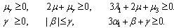
2. Basic Equations
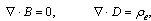
- Here we consider a conducting unsteady flow of an incompressible MHD micropolar conducting fluid, with modified Ohm’s law, of finite conductivity σo, permeated by an initial magnetic field H. This produces an induced magnetic field h and induced electric field E. The basic equations of magnetic and electric fields, continuity, motion, and energy for unsteady flow of micropolar fluids in the presence of a transverse magnetic field with the velocity vector V and the rotation vector ω are:1. The variation of the magnetic and electric fields are given by Maxwell’s equations
 | (1) |
 | (2) |
 | (3) |
 | (4) |
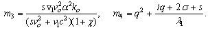
 | (5) |
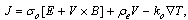
 the coefficient connecting the temperature gradient and electric current and S is the Seebeck coefficient2. The continuity equation has the form:
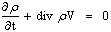 | (6) |
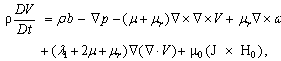 | (7) |
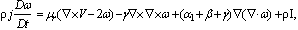 | (8) |
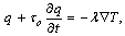
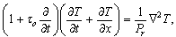
 4. The equation of energy in the absence of heat source is given by:
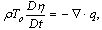 | (9) |
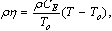 | (10) |
 | (11) |
 defined as
  By eliminating η between (9) and (10) and using (11) we get the equation of heat conduction for the linear theory as follows
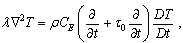 | (12) |
3. Formulation of the Problem
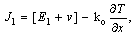
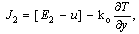
- Our interest here is the case of unsteady two-dimensional flow of an incompressible micropolar conducting fluid past an infinite horizontal moving plate, with modified Ohm's and Fourier’s laws permeated by an initial magnetic field Ho, acting along the z-axis. The velocity components of the fluid are u, and v in the x and y directions, respectively, taken parallel and perpendicular to the plate. We assume the initial magnetic field H, the induced magnetic field , the induced electric field E which is normal to the considered magnetic field, and the electric current density J is parallel to the electric field as H = (0, 0, Ho), h = (0, 0, h), E = (E1, E2, 0), and J = (J1, J2, 0), and the microrotation in z- axis ω = (0, 0, ω). Since the system (1)-(8) and (11) is nonlinear; we come across certain difficulties during its investigation. On the other hand, to solve many problems of applied nature it is sufficient to consider a linearized variant of the system (1)-(8). The equations of Navier-Stokes can be linearized by two well-known methods: that of Stokes and that of Oseen. When using Stokes' method of linearization, nonlinear terms are totally discarded. This method yields satisfactory results for small V, ω and T (note that in this case nonlinear terms are small values of higher order). However, if the fluid flow velocity V is not a small value, this model leads to an essential error. In particular, the effects predicted by this method when a fluid flows along a solid body do not agree with experimental data.A lesser error is obtained in the case of linearization by Oseen's method consisting in the following: it is assumed that fluid flow differs but little from flow along the x-axis with constant velocity v0. Then we set
 [23,24].Under these assumptions, the vector system (1)-(8) and (11) reduces to an Oseen-linearized system of scalar equations of a MHD micropolar conducting fluid with modified Ohm's law in two-dimensional case:
 | (13) |
 | (14) |
 | (15) |
 | (16) |
 | (17) |
 | (18) |
 | (19) |
 | (20) |
 | (21) |
 | (22) |
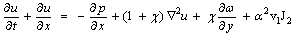
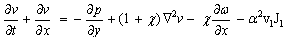
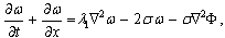
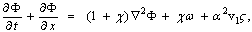
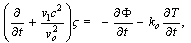
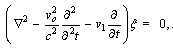
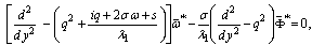
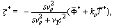
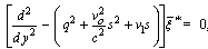
 For simplifications the above equations we have used the following non-dimensional variables (dropping the asterisks for convenience):Differentiating Eq. (14) with respect to x and Eq. (15) with respect to y, and then adding these two equations, we obtain
 | (23) |
 | (24) |
 | (25) |
 | (26) |
 is a two dimensional Laplace operator,
  is the stream function satisfying the continuity equation with
 | (27a) |
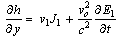
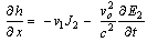
 the potential functions of current density defined by
 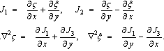 | (27b) |
4. Formulation and Solution in the Laplace and Fourier Transforms Domain
- Applying Laplace and Fourier transforms, respectively defined by the relations

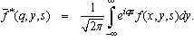 of both sides of Eqs. (24)–(26), (16), and (17) we get
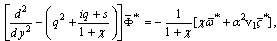 | (28) |
 | (29) |
 | (30) |
 | (31) |
 | (32) |
 between Eq. (31) and (28), we obtain
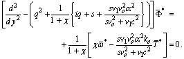 | (33) |
 we should suppress the positive exponential which are unbounded at infinity. The solution of Eq. (30), and (32) can be written as
 | (34) |
 | (35) |
 Eliminating
  and
and  between Eqs. (29), (30) and (33) we arrive at the following fourth order differential equation satisfied by
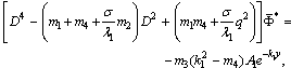 | (36) |
 The solution of Eq. (36) can be written
 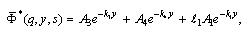 | (37) |
 and
and ,
, are the roots of the characteristic equation
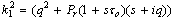
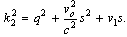
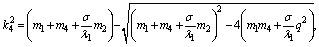
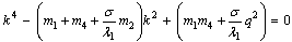 These roots are given by
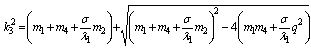 ,
, Eliminating
  and
and  between Eqs. (29), (30) and (33), we find that
 satisfy the same equation as
 i.e
i.e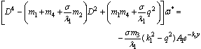 | (38) |
 | (39) |
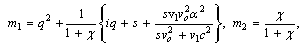
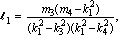
 . The compatibility between these equations and Eqs. (37) and (29), give
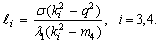 Through out the equations (34) and (37), we can obtain the other component of current density potential functions
 :
:  | (40) |
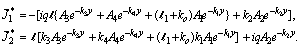
 By Applying Laplace and Fourier transforms of both sides of Eqs (27) and by substituting into Eqs (35), (37) and (40) we can obtain the velocity and current density components as follows:
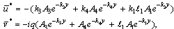 | (41) |
 | (42) |
 | (43) |
 | (44) |
 | (45) |
 | (46) |
5. Applications
- We shall consider unsteady two-dimensional flow of an incompressible micropolar conducting fluid past an infinite horizontal plane surface in the presence of a induced magnetic field occupying the region
 of the space. Choosing the y-axis perpendicular to the surface of the plate with the origin coinciding with the middle plate, the region Ω under consideration becomes
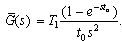
 (1) Thermal boundary condition The boundary of the half-space is affected by ramp-type heating, which depends on the coordinate x and the time t of the form
 | (47) |
 | (48) |
 | (49) |
 (2) Mechanical boundary conditionsWe assume that, the plate is moving with velocity vo and non-conducting surface. The transverse components of the electric field intensity are continuous across the surface of the half-space. This leads to:
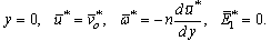 | (50) |
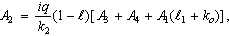
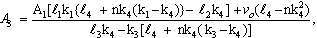
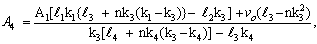
 , where the case n = 0 is called strong concentration by Guram and Smith[22], indicates ω = 0 near the wall and represents concentrated particle flows in which the microelements close to the wall surface are unable to rotate (Jena and Mathur[26]). The case n = 1/2 indicates the vanishing of anti-symmetrical part of the stress tensor and denotes weak concentration (Ahmadi[27]). The case n = 1, as suggested by Peddieson[28], is used for the modeling of turbulent boundary-layer flows.With the help of equations (34), (39), (41), (44), (49) and (50) we obtained
6. Inversion of the Transforms
- To obtain the solution of the problem in the physical domain (x,y, t), we have to invert the iterated transforms in Eqs. (41)–(46). These expressions can be formally expressed as functions of x and the parameter of the Fourier and Laplace transforms q and s of the form
 .First, we invert the Fourier transform using the inversion formula given previously. This gives the Laplace transform expression
  of the function f(x,y, t) as
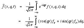 where fe and fo denote the even and the odd parts of the function
  respectively.We shall now outline the numerical inversion method used to find the solution in the physical domain. For fixed values of x, y, and q the function inside braces in the last integral can be considered as a Laplace transform
  of some function g(t).The inversion formula for the Laplace transform can be written as
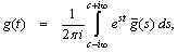 where c is an arbitrary real number greater than all the parts of the singularities
 . Taking s = c + iy, the above integral takes the form
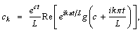
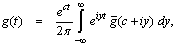 Expanding the function h(t) = exp(-ct)g(t) in a Fourier series in the interval[0, 2L], we obtain the approximate formula.
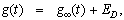 Where
Where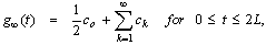 | (51) |
 | (52) |
 | (53) |
 where the discretization error
 . Thus, the approximate value of g(t) becomes
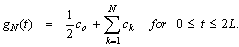
 | (54) |
 be the sequence of partial sums of Eq. (53). We define the e-sequence by
 and
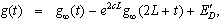
and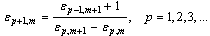 it can be shown that the sequence ε1,1, ε3,1, ε5,1, ..., εN,1, converges to f(x,y, t) + ED – co/2 faster than the sequence of partial sums sm (m = 1,2,3,...).The actual procedure used to invert the Laplace transform consists of using Eq. (67) together with the ε-algorithm. The values of c and L are chosen according to the criteria outlined Honig and Hirdes[29].
7. Results and Discussion
- The purpose of this section is to see the influence of some interesting parameters on the horizontal, normal velocity, microrotation and transverse electric fields. In particular, attention has been focused to modified Ohm’s law (ko parameter) and Alfven velocity parameter α in two cases the first for strong concentration (n=0) and the other for weak concentration (n=1/2), many previous studies of conventional and conjugate problems did not consider this parameter, on the horizontal and normal velocity. The effect of Prandtl number Pr, ramp-type heating parameter to and modified Fourier law’s (relaxation time τo) are also investigated on the temperature. The distribution of non- dimensional temperature T, non-dimensional horizontal velocity u, non-dimensional normal velocity v, non-dimensional micro-rotation ω, and non-dimensional transverse electric field E1 with non-dimensional distance y have been shown in Figs. 1–12. Numerical analysis has been carried out by taking x range from 0 to 1for strong concentration and from 0 to 3 for weak concentration. The computations are carried out for the non-dimensional time t=1.5 and non-dimensional x = 2.The field quantities, velocity, microrotation and electric fields do not depend only on the state and space variables t , x and y, but also depend on ko and Alfven velocity parameters. It has been observed that, these parameters play a vital role on velocity, microrotation and electric fields. The numerical values for the field temperature are computed for a wide range of values of finite pulse rise-time to in the two situations t > to and t < to and relaxation time τo=0.2.
 | Figure 1. Horizontal velocity profiles vs. y for different values of k0 and v0 for strong concentration (n=0) |
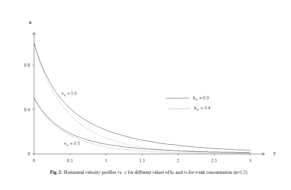 | Figure 2. Horizontal velocity profiles vs. y for different values of k0 and v0 for weak concentration (n=1/2) |
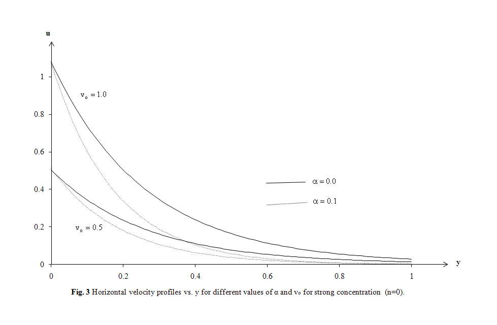 | Figure 3. Horizontal velocity profiles vs. y for different values of α and v0 for strong concentration (n=0) |
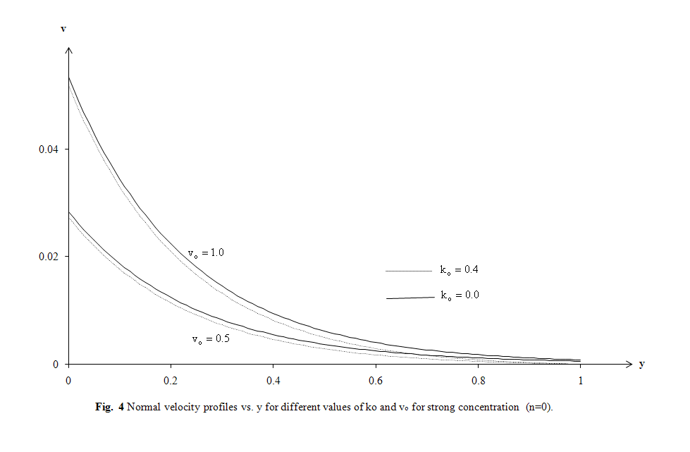 | Figure 4. Normal velocity profiles vs. y for different values of k0 and v0 for strong concentration (n=0) |
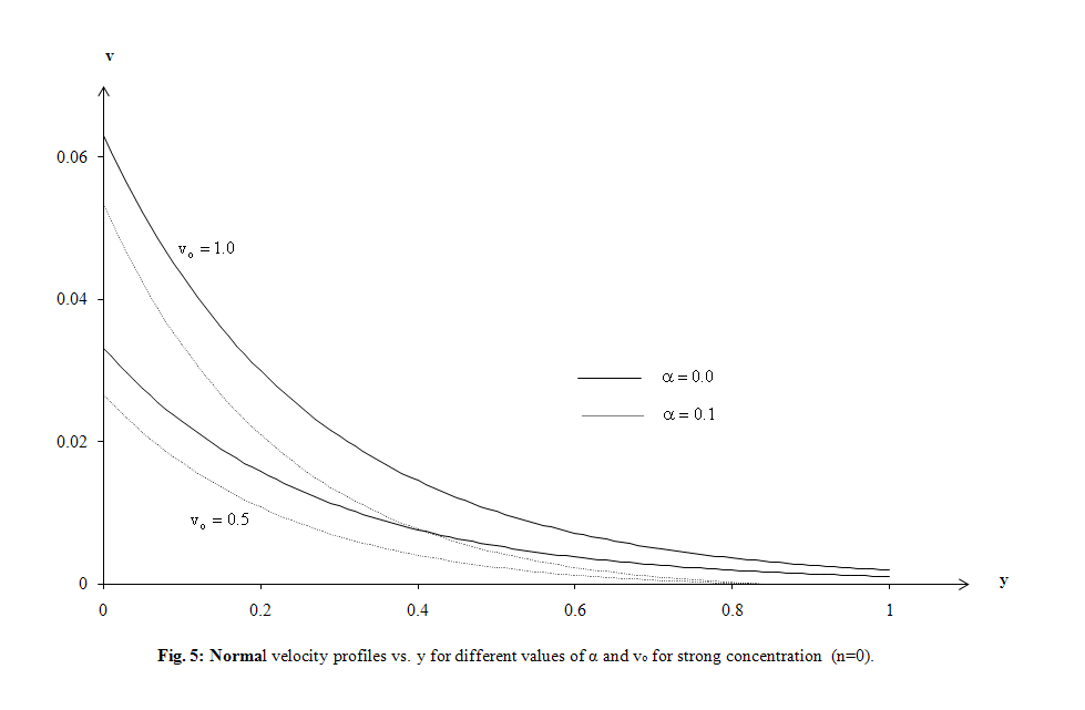 | Figure 5. Normal velocity profiles vs. y for different values of α and v0 for strong concentration (n=0) |
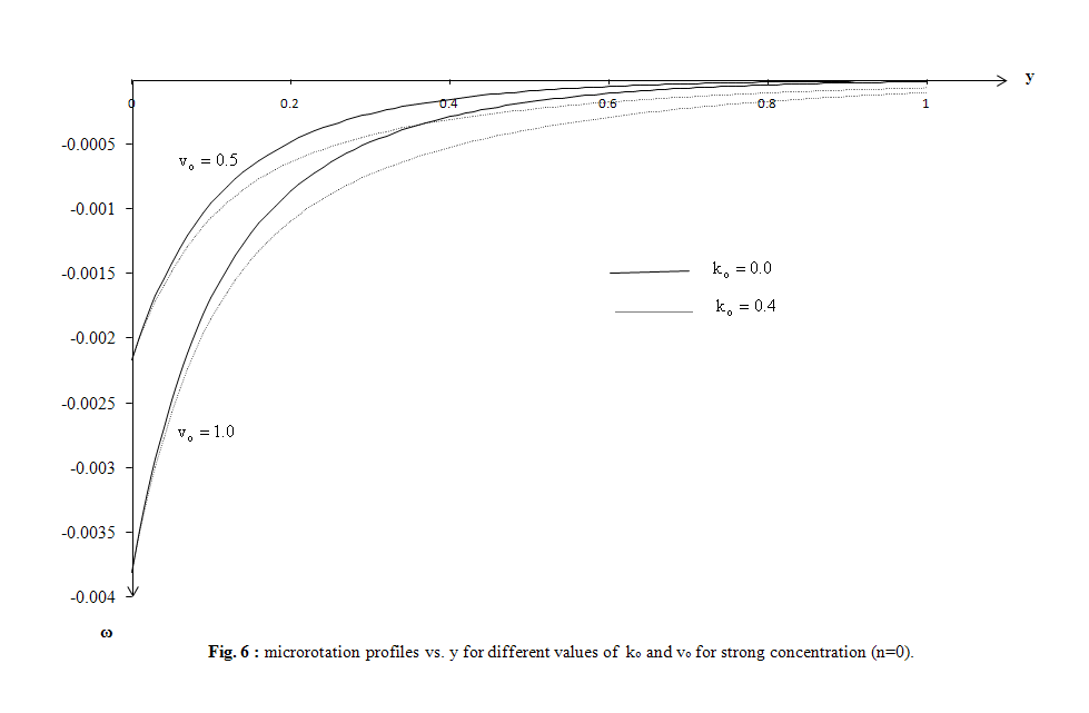 | Figure 6. microrotation profiles vs. y for different values of k0 and v0 for strong concentration (n=0) |
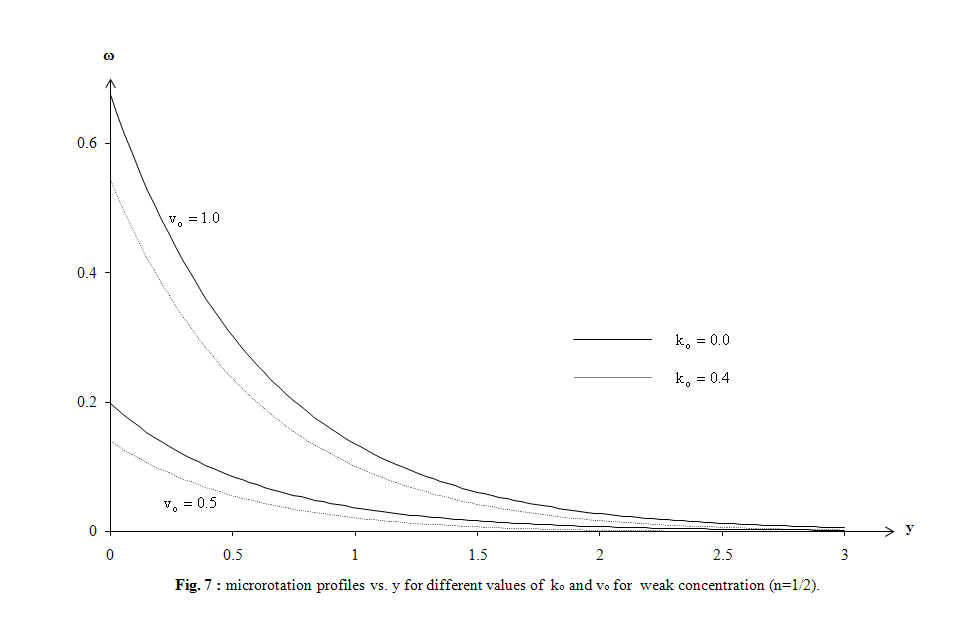 | Figure 7. microrotation profiles vs. y for different values of k0 and v0 for weak concentration (n=1/2) |
 | Figure 8. microrotation profiles vs. y for different values of α and v0 for strong concentration (n=0) |
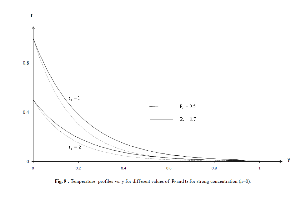 | Figure 9. Temperature profiles vs. y for different values of Pr and to for strong concentration (n=0) |
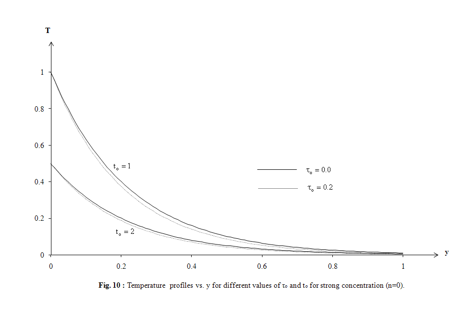 | Figure 10. Temperature profiles vs. y for different values of τo and to for strong concentration (n=0) |
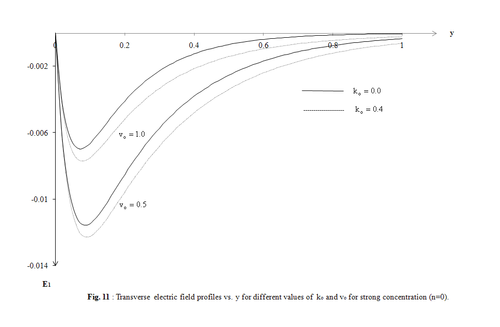 | Figure 11. Transverse electric field profiles vs. y for different values of ko and vo for strong concentration (n=0) |
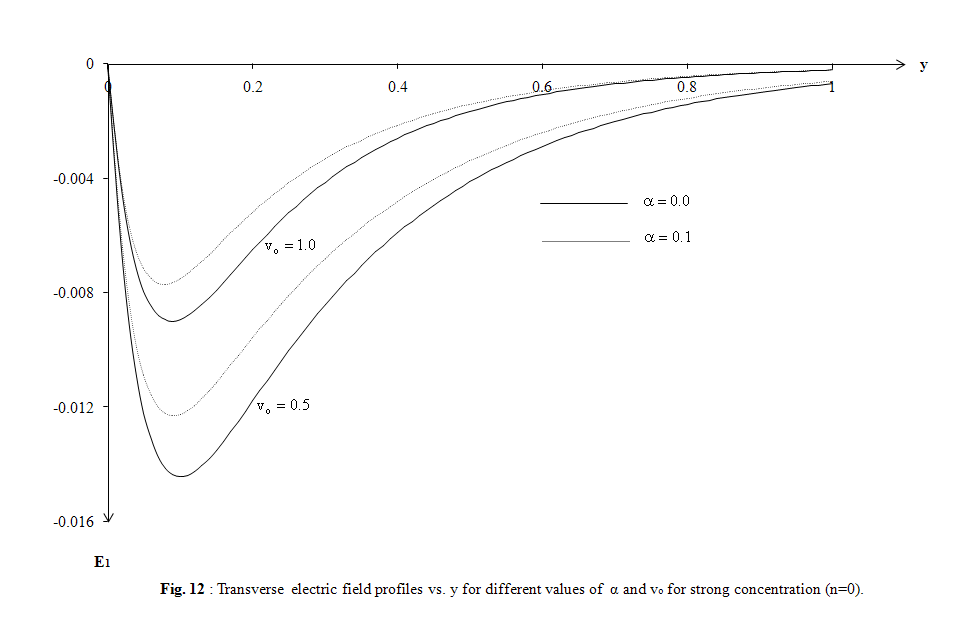 | Figure 12. Transverse electric field profiles vs. y for different values of α and vo for strong concentration (n=0) |
8. Conclusions
- The trend of variations of the temperature distribution T, horizontal velocity u, normal velocity v, horizontal conduction current density component J1 normal conduction current density component J2, and microrotation vector ω are quite different on the application of new model and old model. The medium which are taken is affected by parameters ko , τo and magnetic field, more on the application of modified Ohm’s and Fourier’s laws in comparison to the application of classical model. The increasing in the values of temperature may be explained as the lost heat generating from the movement of electric current, this heat may be the main reason to make that the deformation of the micropolar fluid tends to be normal while the components of electric and magnetic fields record values greater than the values recorded in the old model.
Nomenclature
- ∇ del operatorH magnetic intensity vectorJ conduction current density vectorD electric flux vectorE electric intensity vectorB magnetic flux vectorρe charge densityμo magnetic permeabilityεo electric permittivityσo electric conductivityV velocity vectorT temperature of the fluidTo mean temperature of the surfaceρ density of the fluidCE specific heat at constant pressureλ thermal conductivityq heat flux vectorτo relaxation timeμ shear kinematic viscosityb body force per unit massω microrotation vectorj gyration parametersμr coupling viscosity coefficient or vortex viscosityI body couple per unit massα2=
 , Alfven velocityν kinematic viscosityνr kinematic coupling viscosity
 temperature far away from the surfacep fluid pressureU free stream velocityPr Prandtl numberc speed of light = 1/