1. Introduction

Stirred tanks have wide applications in different industrial process. In the various applications, stirred tanks are required to fulfill several needs like blending of miscible liquids, dispersion of gases or immiscible liquids into a liquid phase, suspension of solid particles, heat and mass transfer promotion and chemical reactions. The study of the hydrodynamic structure generated in stirred vessels is interesting to improve the performances of the agitators and the vessels by the development of the geometrical and operational conditions[1-3]. In the literature, the study of the hydrodynamic structure generated with a pitched blade turbine (PBT) was initiated in several experimental and numerical works on the discharge zone. For example, we can cite the experimental works of Nagata[4], Suzukawa et al.[5], Karcz et al.[6], Dan Taca et al.[7], Armenante et al.[8], and Aubin et al.[9]. In his experimental study, Nagata[4] studied the effect of the pitched blades on the power number with two pitched blades turbine (PBT2). Using a LDA system, Suzukawa et al.[5] studied the effect of the pitched blades in a baffled stirred tank equipped with a four pitched blade turbine (PBT4). Karcz et al.[6] studied the influence of the baffles on the variation of the power number with a three pitched blades turbine (PBT3). Moreover, Armenante et al.[8] studied the hydrodynamic structure of the turbulent flow generated with a six pitched blades turbine (PBT6) is investigated for two

View the lack of the numerical results to predict the effect of the tank design on the hydrodynamic behavior with a PBT6 turbine, we focus on three different systems characterized by cylindrical, curved and spherical tanks. Particularly, we present the evolution of the velocity fields and the turbulent characteristics in different planes. Also, we calculate the power number in each stirred tanks.

2. Stirred Vessels Configuration

In this paper, we have studied the effect of the tank design on the turbulent flow pattern. Three types of tank; a cylindrical tank, a curved tank and a spherical tank; have been equipped with a pitched blade turbine (PBT6). The first system configuration is similar to Armenante et al.[8] application (Figure 1.a). This configuration is characterized by a cylindrical tank equipped with a six pitched blade turbine PBT6. The inclined angle of the blade is equal to β=45°. This turbine have a diameter equal to d=D/3 and is placed in an axial position equal to z=H/4. The tank diameter D is equal to its height H (D=H).

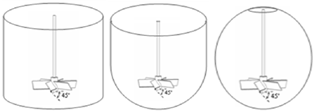Figure 1. Stirred tanks configurations

3. Numerical Model

The CFD code "Fluent" is used for numerical simulation of hydrodynamic structure of turbulent flows in a stirred tank. This code is based on solving Navier-Stokes equations with a finite volume discretization method described in detail by Patankar[15]. This technique consists in dividing the computational domain into elementary volumes around each node in the grid; it ensures the flow continuity between nodes. The spatial discretization is obtained by following a procedure for tetrahedral interpolation scheme. As for the temporal discretization, the implicit formulation is adopted. The transport equation is integrated over the control volume. The algorithm SIMPLE is used for pressure velocity coupling. To model the geometry of the impeller exactly, a 3D simulation is performed. The Multi Reference Frame (MRF) approach is available to incorporate the motion of the impeller in the stirred tank. This steady-state approach allows modelling the baffled stirred tanks and the tanks with other complex internals. It’s recommended for simulation by the several searchers like Armenante et al.[8], Vakili et al.[13], Luo et al.[16], Akiti and Armenante[17] and Deglon and Meyer[18]. The grid used for the MRF solution should have a perfect surface of revolution surrounding each rotating frame. The rotating frame is used for the region containing the rotating components while a stationary frame is used for the stationary regions. The momentum equations, inside the rotating frame, are solved in the frame of the enclosed impeller while the rotating frame is solved in the stationary frame. A steady transfer of information is made at the MRF interface as the solution progresses.

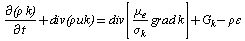
3.1. Governing Equations

The equations to be solved are the continuity and momentum equations. The continuity equation is a statement of conservation of mass for a constant density fluid, it takes the form:

(1)

The momentum equations are a statement of conservation of momentum in each of the three components. The three momentum equations are collectively called the Navier-Stokes equations. In addition to momentum transport by convection and diffusion, several momentum sources are also involved. The momentum equations take the form:

(2)

The total pressure p is defined by the following equation:

(3)

The k-ε model is one of a family of two-equation models, for which two additional transport equations must be solved in order to compute the Reynolds stresses. The RNG k-ε model was developed in response to the empirical nature of the standard k-ε model. Rather than being based on observed fluid behavior, it is derived using statistical methods used in the field of renormalization group (RNG) theory. It is similar in form to the standard k-ε model, but it contains modifications in the dissipation equation to better describe flows with regions of high strain. In addition, a differential equation is solved for the turbulent viscosity. This model is used by several authors such as Montante et al.[19], Jaworski and Zakrazewska[20], Launder[21], Orszag and Yakhot[22] and Kelly and Gigas[23].

The equation of the turbulent kinetic energy is given in the following form:

(4)

The equation of the dissipation rate of the turbulent kinetic energy is written as follow:

(5)

G_k is the turbulent kinetic energy production term:

(6)

The effective viscosity is defined as follow:

(7)

Where, is the turbulent viscosity defined as follow:

(8)

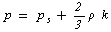
3.2. Power Dissipation

The knowledge of the power consumption is very important for the choice of the system installed. The power consumption depends on all parameters characterizing the external geometry of the tank, the geometry of the agitator, the flow regime and the rotating speed of the mobile. The power number Np allows to extrapolate calculations of the power when the diameter of the agitator d and its rotational speed N change. The power number is defined as follow:

(9)

P is the power consumption of the agitator system, given by:

(10)

Where, C is the torque of the agitator system.

4. Numerical Results

The numerical results are presented in the entire tank. Using the MRF steady-state approach, the distribution of the velocity fields and the turbulence characteristics have been introduced in the vertical and horizontal planes containing the blade. The turbulent flow is defined by a Reynolds number Re=71000. Due to the symmetry of the system, the computational domain is reduced to 60°, which includes one blade. At the two frontal planes defined by angular positions θ=±30°, periodic conditions are imposed on all properties ensuring the continuity of the computational domain in the angular direction. A typical simulation is considered converged when the residual mass and other quantities characterizing the flow as the three velocity components and turbulent kinetic energy and the dissipation rate fall below 10-6 [24].

4.1. Flow patterns in r-z plane

Figure 2 presents the flow pattern in vertical plane containing the blade. In these tanks, it’s noted that the pitched blades turbine generates a radial jet developed from the blade and propagates in the lower part of the tank. At the proximity of the sidewall, the radial jet has been transformed into two axial jets upward and downward. Also, we note the appearance of a recirculation loop located in the upper zone of the tank. At the curved bottom of the tank, a secondary recirculation loop appears just below the turbine. Beyond the area swept by the turbine, the mean velocity decreases gradually and becomes very low at the top of the cylindrical tank.

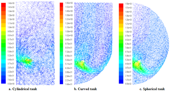Figure 2. Flow patterns in r-z plane

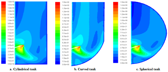Figure 3. Distribution of the mean velocity in r-z plane

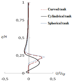
Figure 4. Radial profiles of the axial velocity component

4.2. Mean Velocity in r-z Plane

Figure 3 presents the distribution of the mean velocity in the vertical plane containing the blade. Globally, it’s noted that the appearance of the maximum values wake developed in the area swept by the turbine. Moreover, we find that the mean velocity decreases gradually away from the pitched blade turbine and becomes very low at the bottom and at the top of the tank. The discharge jet is more intense in the curved tank and it reaches the sidewall. The recirculation loop is more extended in the upper part of this tank and reduces the stagnant fluid zone. At the curved bottom, the second recirculation loop is appeared in the lower part of the curved tank that proves a significant fluid circulation. With a curved bottom, we observe total disappearance of the dead zones initially located at the bottom of the cylindrical tank. Contrary to the spherical tank, in the upper part the dead zones have been more developed and the recirculation loop is located near the turbine that proves the decrease of the fluid motion. Thus, we can deduce that the curved bottom reduces the stagnant areas and promotes more uniformity throughout the volume of the tank without having to modify the external geometry of the upper surface of the tank.

4.3. Radial Profiles of the Axial Velocity Component

Figure 4 shows the radial profiles of the axial velocity component in r-z plane containing the blade for different axial position defined by z/H=0.18, z/H=0.24, z/H=0.31, z/H=0.55 and z/H=0.79. Globally, these profiles show a great resemblance between them. The axial component vanishes at the sidewall of the tank (2r/D=1) and at the shaft (2r/D=0). Between two axial positions, these profiles follow a variation between the maximum and the minimum values. In the turbine area, these profiles present a minimum for the axial component due to the downward flow aspired by the rotation motion of the turbine. At the sidewall, these profiles reverse and reach the maximum which proves the existence of the axial upward jet. At the top of the curved tank, the axial velocity component becomes very intense. Also, at the bottom of the curved tank, the axial velocity component is very important to compare with the two other systems. So, we can deduce that the curved tank creates a largest fluid circulation. Figure 4.a shows a good agreement between our numerical results found in the case of a cylindrical tank, with experimental results found by Armenante et al.[8], which proves the validity of the numerical method adopted.

4.4. Axial Profiles of the Radial Velocity Components

Figure 5 shows the axial profiles of the radial velocity component in the vertical plane containing the turbine. These profiles are presented on the height of the tank in front of the blade end. Globally, it’s noted that the radial velocity component vanishes in the lower part of the curved bottom of the second and third tank. But, in the case of a cylindrical tank, the negative values shown in the lower part of the tank prove the existence of the small recirculation loop below the pitched blade turbine. The radial component is maximal in the discharge jet of the turbine. The negatives values of the radial component prove the existence of the recirculation loop just above the turbine and it vanishes in the top of each tank. We can deduce that the design of the upper part has no effect on the evolution of the radial velocity component.

Figure 5. Axial profile of the radial velocity

4.5. Axial Profiles of the Tangential Velocity Components

Figure 6 presents the axial profiles of the tangential velocity component in the vertical plane containing the turbine. These profiles are presented on the height of the tank in front of the blade end. Globally, we can distinct three zones. The discharge zone characterized by a maximum values of the tangential component is located between two axial positions equal to z/H=0.17 and z/H=0.34. Below the turbine, the tangential component is very important. This fact proves the existence of a centrifugal fluid flow. Thus, the design of the bottom has a direct effect on the tangential component. With a curved bottom, the tangential component increases in the discharge area of the turbine and also in the lower area of the tank. It decreases gradually at the upper part and it vanishes in proximity of the spherical tank top surface. Then, we can deduce that the curved tank promotes more fluid circulation throughout the volume.

Figure 6. Axial profiles of the tangential velocity

4.6. Turbulent Kinetic Energy in r-z Plane

Figure 7 presents the distribution of the turbulent kinetic energy in the vertical plane containing the blade. In the each system, the wake of the maximum values of the turbulent kinetic energy appears on the mechanical source and develops within the fluid to reaches the sidewall of the tank. Also, it’s noted that the turbulent kinetic energy is more extended in the case of the spherical tank.

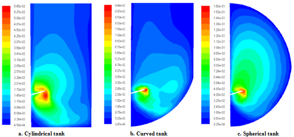Figure 7. Distribution of the turbulent kinetic energy in r-z plane

Figure 8. Radial profiles of the turbulent kinetic energy

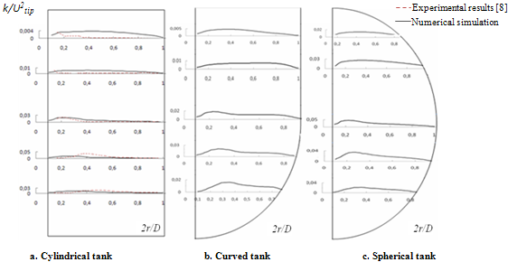
4.7. Radial Profiles of the Turbulent Kinetic Energy

Figure 8 shows the radial profiles of the turbulent kinetic energy in r-z plane containing the blade. These profiles present the evolution of the turbulent kinetic energy in each system in different axial positions defined by z/H=0.18, z/H=0.24, z/H=0.31, z/H=0.55 and z/H=0.79. Globally, we observe a great similarity between these profiles. The turbulent kinetic energy vanishes at the sidewall of the tank (2r/D=1) and at the shaft (2r/D=0). Between these axial positions, the turbulent kinetic energy is maximal in the area swept by the PBT6 turbine and decreases gradually outside the discharge jet of the turbine. Figure 8.a shows a good agreement between our numerical results found in the case of a cylindrical tank with experimental results found by Armenante et al.[8], which proves the validity of the adopted numerical method.

4.8. Axial Profiles of the Turbulent Kinetic Energy

Figure 9 shows the axial profiles of the turbulent kinetic energy in the vertical plane containing the blade. According

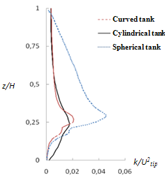Figure 9. Axial profiles of the turbulent kinetic energy

4.9. Dissipation Rate of the Turbulent Kinetic Energy

5. Global Characteristics

Figure 11 presents the variation of the power number NP depending on the Reynolds number Re with a pitched blade turbine PBT6 placed respectively in the cylindrical, the curved and the spherical tank. Globally, we find that the energy dissipation defined within the fluid increases with the curved bottom of the tank. For the Reynolds numbers between Re=103 and Re=104, the energy dissipation defined in these three systems is very important. In fully turbulent regime, for Reynolds number between Re=104 and Re=105, the curved tank shows a much greater dissipation of energy.

Figure 10. Distribution of the dissipation rate of the turbulent kinetic energy in r-z plane

Therefore, we can deduce that the curved tank is the best system because the presence of the curved bottom improves the quality of the mixture. So, this system consumes slightly more of the energy dissipation than the other systems.

In the case of a cylindrical tank and for the rotating speed Ω=450 rpm, the power number calculated with the CFD code is equal to Np=0.578. This value is close to experimental value Np=0.670 found in the literature by Armenante et al.[8]. This proves the validity of the numerical method adopted.

Figure 11. Evolution of the power number

6. Conclusions

The comparative study has been affected between three different configurations equipped with cylindrical, curved and spherical tank. Specifically, we have studied the effect of the tank design on the hydrodynamic structure of the turbulent flows generated by a six-pitched blade turbine (PBT6). The velocity components and the turbulent characteristics have been presented in different planes containing the blade. We can deduce that the use of the pitched blade turbines in the curved tank can increase the pumping action in the full tank, with slightly higher energy. In the future, we propose to characterise the hydrodynamic structure of this turbine by the particle image velocimetry (PIV) experimental technique.

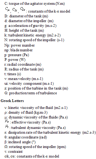
Nomenclature