Gopinath Subramanian
School of Polymers and High Performance Materials, University of Southern Mississippi, Hattiesburg, USA
Correspondence to: Gopinath Subramanian, School of Polymers and High Performance Materials, University of Southern Mississippi, Hattiesburg, USA.
| Email: |  |
Copyright © 2015 Scientific & Academic Publishing. All Rights Reserved.
Abstract
An analytical approximation for the probability density function of a one-dimensional random walk with gradually varying step sizes is derived using the convolution theorem for Fourier transforms. The range of applicability of this expression is studied by numerical simulations for the particular case of strictly decreasing step sizes.
Keywords:
Random walks, Polymers, Approximation
Cite this paper: Gopinath Subramanian, A Note on Random Walks with Varying Step Sizes, American Journal of Materials Science, Vol. 5 No. 2, 2015, pp. 53-56. doi: 10.5923/j.materials.20150502.05.
1. Introduction
The random walk, a term coined by Pearson [1], finds utility in an incredible number of scientific and technological fields, ranging from polymer physics [2] and biology [3] to the “who-to-follow” algorithm used by the popular social networking website Twitter [4]. A one-dimensional random walk is a path traced by a walker that takes a succession of steps, with each step chosen with equal probability to be either to the left or to the right. The overwhelming majority of analyses assume, for simplicity, that the step length of a random walker remains constant throughout the duration of the random walk. However, this need not always be the case and studies of random walks with monotonically decreasing step size, referred to as Bernoulli convolutions, are available in the mathematics literature [5, 6, 7, 8, 9]. Random walks with monotonically increasing step size, referred to as greedy random walks, have also been studied [10]. In both these types of studies, the random walk is discretized into a sequence of steps and the step size is changed at every step. In the case of Bernoulli convolutions, the step size is a strictly decreasing function of step number, while in the case of greedy random walks, it is a strictly increasing function.In this note, I examine a slightly different type of random walk where the step size is held constant for a sufficiently large number of steps,  before it is changed. This problem lends itself to a simplified analysis, and yields a closed-form solution for the probability density function (PDF) of the end-to-end vector, and consequently, other quantities of interest such as the hydrodynamic radius. The analytical solution is compared with numerical simulations of random walks in order to assess the limits of its applicability. One potential application is in the field of gradient copolymers, where the polymer stiffness varies gradually along the backbone, such as the sinusoidal variation produced by Lefebvre et al. [11] Another application would be in diffusivity problems, where the diffusivity of a particle is a function of time, or if a particle were diffusing in a temperature gradient.
2. Formulation
A one-dimensional random walk is first discretized into a sequence of blocks, where the  block is made up of
  steps of size
  and each individual step is either
  or
or For simplicity, the step size of the first block is set to
 Figure 1 shows, for the particular case of strictly decreasing step sizes, a plot of step size as a function of step number with two different block sizes, viz.,
  (which is equivalent to changing step sizes at every step) and
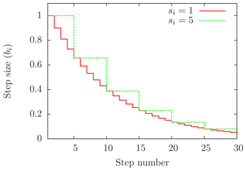 | Figure 1. A random walk is discretized into a sequence of blocks. Each block contains  steps of equal length. The case where steps of equal length. The case where shown with the solid red line, is equivalent to having the step length change at every step shown with the solid red line, is equivalent to having the step length change at every step |
If we shift the origin so that it is at the position of the walker before it begins the  block, and if the number of steps of the
  block is sufficiently large, the PDF of the end-to-end distance of a one-dimensional random walker is given by a Gaussian with zero mean and variance
  as [12]
  | (1) |
For a sequence of two blocks, the PDF of the end-to-end distance is given by the convolution of the Gaussians for each block as  | (2) |
It can be shown using the convolution theorem for Fourier transforms that the convolution of two normalized Gaussians, say  and
and  is another normalized Gaussian. The resultant Gaussian also has the useful property that its mean and variance are respectively equal to the sum of the means and the sum of the variances of the individual Gaussians. In other words,
  | (3) |
 | (4) |
This result can be extended to an arbitrary number of Gaussians. For the 1-D random walk under consideration, the PDF of the end-to-end distance after  blocks is therefore a Gaussian with zero mean, and a variance equal to the sum of the individual variances, and is given by
  | (5) |
For a continuously varying step length (such as might be encountered in diffusion problems), the replacement of the summation by an integral can be accomplished with relative ease, and will not be discussed here. If we set and
and  for all values of
  equation 5 reduces to the standard Gaussian distribution for the end-to-end distance of a 1-D random walk given by
  | (6) |
3. Comparison with Numerical Simulations of Strictly Decreasing Step Sizes
For comparison with numerical simulations, the individual  were restricted to be equal to a single value,
  and PDFs were computed over
  random walks for a given set of parameters. The error was defined as the integral of the absolute difference between the analytical and numerical PDFs:
 | (7) |
with  | (8) |
The prototypical 1-D random walk with strictly decreasing step sizes has an end-to-end distance given by:  | (9) |
where  is a random variable that can take on values of
  or
or  with equal probability. The PDF of
  is called an infinite Bernoulli convolution [6], which in the language of equation 5, is the PDF of the end-to-end distance of random walks with
 . The worst case scenario for using equation 5 is obtained for infinite Bernoulli convolutions in the limit as
 Here, the random walk effectively terminates after the first step, and the PDF of
  approaches a function which is the mean of two delta functions centered at
 given as:
  | (10) |
where  refers to the Dirac delta function. Denoting the pointwise error as
  | (11) |
where  and
and  are as given in equations 5 and 10 respectively, the error can be computed as an integral over the real line as:
 | (12) |
This integral can be split into the sum of two limits: the first in the neighborhood of  , and the second over the rest of the real line, which is written as:
 | (13) |
In the neighborhood of  does not affect the delta functions. Away from
 , the delta functions do not affect
 Consequently, each of the limits evaluate to unity, yielding
  | (14) |
Random walks with strictly decreasing step sizes were obtained by setting as in the case of Bernoulli convolutions, and a natural end point for this type of random walk is when
  Practically, this is achieved by setting a cutoff step size of
  and terminating the random walk when the step size drops below this threshold. Decreasing the cutoff below this value by two orders of magnitude did not produce any changes in the errors.Figure 2 shows a plot of the actual distributions for infinite Bernoulli convolutions, along with the analytical approximations. Figure 2 (a) is the worst-case scenario with
  For
For the numerical distribution seems to have a self-similar structure, as shown in figure 2(b) and its inset. For
  and
and shown in figure 2(c) and (e), the distributions have a simple form and was shown by Krapivsky and Redner [7] to be the result of a “fortuitous cancellation of errors.” For
  the inverse of the golden ratio, the numerical simulations show the self-similar structure of the distribution, as previously reported [7], and referred to as the “golden walk.”
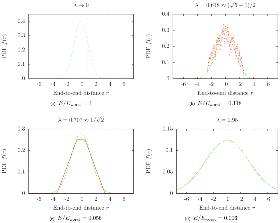 | Figure 2. Comparison between numerical simulations (red points) and the approximation in equation 5 (green broken line) for infinite Bernoulli convolutions, for various values of  The normalized errors are indicated. Note that the ordinates are slightly different for each sub-figure. For The normalized errors are indicated. Note that the ordinates are slightly different for each sub-figure. For  the approximation given by equation 5 is close to the results of the numerical simulations.which will be used to normalize any errors that are computed for comparing results of numerical simulations with equation 5 the approximation given by equation 5 is close to the results of the numerical simulations.which will be used to normalize any errors that are computed for comparing results of numerical simulations with equation 5 |
While the approximation to the PDF given by equation 5 is incapable of capturing the fine structure that the numerical simulations show, as  increases, the structure disappears and the analytical approximation gets better because we start to approach the regime of gradually decreasing step sizes. For
  the match between numerical simulations and the analytical approximation from equation 5 is reasonable, and figure 2 should also give the reader a sense for whether a particular value of
  is acceptable for his/her purposes.Figure 3 shows a plot of the normalized error,
  as a function of
  for a few selected values of
  For
For there is a prominent kink at
 and is the result of the numerical distribution crossing over from the self-similar structure seen in figure 2 (b) to the structure of figure 2 (d). As
  increases, the error progressively decreases, and the analytical expression in equation 5 becomes applicable to a wider range of
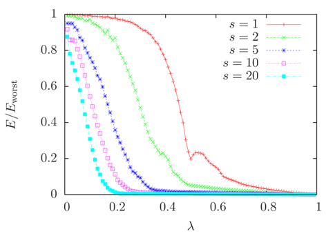 | Figure 3. Normalized error as a function of the step length reduction factor  for various values of block size for various values of block size  . Low values of error are obtained for small . Low values of error are obtained for small  and/or large and/or large  |
ACKNOWLEDGEMENTS
Thanks to Ras Pandey and Bernd Schröder for useful discussions. Support for this work was provided by startup funds from the College of Science and Technology.
References
| [1] | Karl Pearson. “The problem of the random walk.” Nature, 72:294+, 1905. |
| [2] | Werner Kuhn. “Über die gestalt fadenförmiger moleküle in lösungen.” Kolloidzeitschrift, 68:2, 1934. |
| [3] | Howard C. Berg. “Random Walks in Biology.” Princeton University Press, revised edition, September 1993. |
| [4] | Pankaj Gupta, Ashish Goel, Jimmy Lin, Aneesh Sharma, Dong Wang, and Reza Zadeh. “WTF: The who to follow service at twitter.” In Proceedings of the 22Nd International Conference on World Wide Web, WWW ’13, pages 505–514, Republic and Canton of Geneva, Switzerland, 2013. International World Wide Web Conferences Steering Committee. |
| [5] | Richard Kershner and Aurel Wintner. “On symmetric Bernoulli convolutions.” American Journal of Mathematics, 57(3):541+, July 1935. |
| [6] | Paul Erdös. “On a family of symmetric Bernoulli convolutions.” American Journal of Mathematics, 61(4): 974+, October 1939. |
| [7] | "P. L. Krapivsky and S. Redner. “Random walk with shrinking steps.” American Journal of Physics, 72(5): 591–598, May 2004. |
| [8] | Tonguç Rador and Sencer Taneri. “Random walks with shrinking steps: First-passage characteristics.” Physical Review E, 73:036118+, March 2006. |
| [9] | C. A. Serino and S. Redner. “The Pearson walk with shrinking steps in two dimensions.” Journal of Statistical Mechanics: Theory and Experiment, 2010(01):P01006+, January 2010. |
| [10] | E. Ben-Naim and S. Redner. “Winning quick and dirty: the greedy random walk.” Journal of Physics A: Mathematical and General, 37(47):11321+, November 2004. |
| [11] | Michelle D. Lefebvre, Monica Olvera de la Cruz, and Kenneth R. Shull. “Phase segregation in gradient copolymer melts.” Macromolecules, 37(3):1118–1123, 2004. |
| [12] | S. Chandrasekhar. “Stochastic problems in physics and astronomy.” Rev. Mod. Phys., 15:1–89, Jan 1943. |

 before it is changed. This problem lends itself to a simplified analysis, and yields a closed-form solution for the probability density function (PDF) of the end-to-end vector, and consequently, other quantities of interest such as the hydrodynamic radius. The analytical solution is compared with numerical simulations of random walks in order to assess the limits of its applicability. One potential application is in the field of gradient copolymers, where the polymer stiffness varies gradually along the backbone, such as the sinusoidal variation produced by Lefebvre et al. [11] Another application would be in diffusivity problems, where the diffusivity of a particle is a function of time, or if a particle were diffusing in a temperature gradient.
  block is made up of
  steps of size
  and each individual step is either
  or
or For simplicity, the step size of the first block is set to
 Figure 1 shows, for the particular case of strictly decreasing step sizes, a plot of step size as a function of step number with two different block sizes, viz.,
  (which is equivalent to changing step sizes at every step) and
 block, and if the number of steps of the
  block is sufficiently large, the PDF of the end-to-end distance of a one-dimensional random walker is given by a Gaussian with zero mean and variance
  as [12]

 and
and  is another normalized Gaussian. The resultant Gaussian also has the useful property that its mean and variance are respectively equal to the sum of the means and the sum of the variances of the individual Gaussians. In other words,

 blocks is therefore a Gaussian with zero mean, and a variance equal to the sum of the individual variances, and is given by
 and
and  for all values of
  equation 5 reduces to the standard Gaussian distribution for the end-to-end distance of a 1-D random walk given by
 were restricted to be equal to a single value,
  and PDFs were computed over
  random walks for a given set of parameters. The error was defined as the integral of the absolute difference between the analytical and numerical PDFs:


 is a random variable that can take on values of
  or
or  with equal probability. The PDF of
  is called an infinite Bernoulli convolution [6], which in the language of equation 5, is the PDF of the end-to-end distance of random walks with
 . The worst case scenario for using equation 5 is obtained for infinite Bernoulli convolutions in the limit as
 Here, the random walk effectively terminates after the first step, and the PDF of
  approaches a function which is the mean of two delta functions centered at
 given as:
 refers to the Dirac delta function. Denoting the pointwise error as
 and
and  are as given in equations 5 and 10 respectively, the error can be computed as an integral over the real line as:
 , and the second over the rest of the real line, which is written as:
 does not affect the delta functions. Away from
 , the delta functions do not affect
 Consequently, each of the limits evaluate to unity, yielding
 as in the case of Bernoulli convolutions, and a natural end point for this type of random walk is when
  Practically, this is achieved by setting a cutoff step size of
  and terminating the random walk when the step size drops below this threshold. Decreasing the cutoff below this value by two orders of magnitude did not produce any changes in the errors.Figure 2 shows a plot of the actual distributions for infinite Bernoulli convolutions, along with the analytical approximations. Figure 2 (a) is the worst-case scenario with
  For
For the numerical distribution seems to have a self-similar structure, as shown in figure 2(b) and its inset. For
  and
and shown in figure 2(c) and (e), the distributions have a simple form and was shown by Krapivsky and Redner [7] to be the result of a “fortuitous cancellation of errors.” For
  the inverse of the golden ratio, the numerical simulations show the self-similar structure of the distribution, as previously reported [7], and referred to as the “golden walk.”
 increases, the structure disappears and the analytical approximation gets better because we start to approach the regime of gradually decreasing step sizes. For
  the match between numerical simulations and the analytical approximation from equation 5 is reasonable, and figure 2 should also give the reader a sense for whether a particular value of
  is acceptable for his/her purposes.Figure 3 shows a plot of the normalized error,
  as a function of
  for a few selected values of
  For
For there is a prominent kink at
 and is the result of the numerical distribution crossing over from the self-similar structure seen in figure 2 (b) to the structure of figure 2 (d). As
  increases, the error progressively decreases, and the analytical expression in equation 5 becomes applicable to a wider range of

 for various values of block size
  . Low values of error are obtained for small
  and/or large
 Abstract
 Reference
 Full-Text PDF
 Full-text HTML
 steps of equal length. The case where
 shown with the solid red line, is equivalent to having the step length change at every step
 The normalized errors are indicated. Note that the ordinates are slightly different for each sub-figure. For
  the approximation given by equation 5 is close to the results of the numerical simulations.which will be used to normalize any errors that are computed for comparing results of numerical simulations with equation 5