Carl Y. H. Jiang
The Institute for Frontier Materials, Deakin University, Victoria, 3216, Australia
Correspondence to: Carl Y. H. Jiang, The Institute for Frontier Materials, Deakin University, Victoria, 3216, Australia.
| Email: |  |
Copyright © 2012 Scientific & Academic Publishing. All Rights Reserved.
Abstract
A new approach to model adsorption in heterogeneous phase system has been proposed. Three truncated carbon nano tubes and argon are selected as sorbets and sorbent respectively and located into a canonical ensemble which is a cubic box. The length of carbon nano tubes was firstly built by using Hamada index and then the size of cubic box is determined and latticed. The new manner of distributing constant number of fluid particles into cubic box at initial state for an inhomogeneous phase system is randomly distributing particles into the spatial space without touching solid phase. The new approach is not only saving a lot of computational time but also new algorithms are generated so that trajectories of fluid particles can be traced in detail in pursuit of Monte Carlo simulation. Based on a number of fluid particles appears in specific domains, adsorption and desorption can be dynamically defined. In above approach, the interaction energy was calculated by Lennard-Jones 12-6 potential equation, rejection or acceptance of each fluid particle trial was assessed by Boltzmann factor according to Metropolis method.
Keywords:
Monte carlo simulation, Adsorption, Carbon nano tube, Canonical ensemble, Statistical mechanics, Statistical thermodynamics, Computational nanoscience
Cite this paper: Carl Y. H. Jiang, A New Approach to Model Adsorption in Heterogeneous Phase System with Monte Carlo Method, American Journal of Materials Science, Vol. 4 No. 1, 2014, pp. 25-38. doi: 10.5923/j.materials.20140401.05.
1. Introduction
Monte Carlo simulation has been applied into investigating science of adsorption for many years. In terms of different cases, Monte Carlo simulation is often carried out based on different ensemble with different parameter conditions. The feature studies of Vapour - fluid, fluid -fluid and solid phase have been performed by researchers[1-9] respectively. It has been discovered a fact that, for a homogenous phase system, the most of results gained by Monte Carlo simulation satisfies with experimental results. However, for a heterogeneous phase system, macro thermodynamic properties represented in grand ensemble cannot directly be achieved from canonical and microcanonical ensemble as the treatment was made for a homogenous phase system in the traditional manner.On the other hand, researchers have already realized a fact that new algorithms must be created for one specific heterogeneous phase system when Monte Carlo simulation is used by selecting one desired ensemble. In investigating adsorption happening inside pore or one split sorbate, the sorbent treated as particles is initially and fully distributed onto the inner lattices which are already made inside pore or space inside split sorbate. Then interaction energy between fluid particles and solid-phase atoms is based on already made distance[10].However, the main drawback for such a treatment is that 1. It completely ignores radius of pore and the size of split space. In fact, not all fluid particles are able to fill in the spatial space in pores or split sorbate 2. It is difficult to lattice spatial space inside them especially for irregular shape.3. It needs expensive computational time. Features of This ResearchIn order to overcome above defects, a new approach is proposed in the research. The new manner is that 1. Three carbon nano tubes are selected as sorbates;2. The noble gas argon (Ar) is selected as sorbent and treated as fluid particles;3. Both sorbate and sorbent are investigated in canonical ensemble which is made from a cubic box;4. The cubic box is latticed; 5. Fluid particles are randomly distributed into a spatial space;6. The interaction energy between a carbon atom and an absorbed Ar, and Ar-Ar is calculated respectively in the heterogeneous phase system;7. The rejection or acceptance for each fluid particle’s trial is assessed by Boltzmann factor using Metropolis method.
2. Fundamentals of Statistical Thermodynamics
2.1. Canonical Ensemble and Body Energy
In a canonical ensemble, the number of particles N, the system’s volume V, and the system's temperature T are fixed. For a small subsystem which is also called a body, the canonical ensemble is a collection of N identical particles in a volume V at the temperature T in thermal equilibrium with its environment. The total energy of a body E consists of three parts: kinetic energy, external energy and interaction energy. The total energy is then expressed as[11] | (1) |
Where• The first term at the right hand of equation(1) is kinetic energy. • The second term is external energy which is influenced by an external field (such as gravitational, electromagnetic field, etc.). r is the radius of particle i.The third term is interaction energy.• ri and Pi is radius and momentum of particle i with identical mass m respectively.Therefore, for a 6N-dimensional phase space, the state of the body can be characterized by the point (rN,pN) in the form of vector.Because canonical ensemble describes a system in thermal equilibrium with its environment, the heat exchange could exist. The thermodynamic properties can be described microscopic features. The Helmholtz free energy in canonical ensemble can be expressed as follows. | (2) |
where  is the called the canonical partition function for the system of N particles and
  is the thermal de Broglie wavelength of a particle and
  is called a configuration integral with
 | (3) |
kB is Boltzmann constant (1.38066×10⁻²³ J/K); ℏ is Planck’s constant (6.62608×10⁻³⁴J∙s).From above partition function, it can be discovered that the distribution for determining configuration rN of a system has the following correlation.  | (4) |
Where, the potential energy is the sum of pairwise potential terms: | (5) |
The term exp[-βU(rN)] in the correlation(4) is Boltzmann factor over all possible microscopic states. The subscript i and j represent different fluid particles respectively. The particle i and j have identical physical properties, however, in order to easily calculate, they are distinguished one by one. Monte Carlo simulation in canonical ensemble is based on equation(4).In practice, the first term at the right hand of equation(5) can be extended to calculate the fluid-solid interaction energy as well except for calculating fluid-fluid interaction energy. In this research, the second term at the right hand of equation(5) is not considered. Thus, the total potential energy in a heterogeneous phase system consists of two parts:• The sum of potential energy between fluid particle i and j.• The sum of potential energy between fluid particle i and all of the carbon atoms. Which can be written as  | (6) |
Where, rg is the distance separating the adsorbed Argon from the carbon atom g and is a parameter which is difficult to be determined for a heterogeneous phase system. A special technique is to be proposed and introduced in the subsection later.
2.2. Metropolis Algorithm Based Monte Carlo Simulation in Canonical Ensemble
Metropolis Algorithm is to consider the features of fluid particles in microscopic state mentioned above into a cubic volume V with length L. In order to sample and correlate distribution of particles with potential energy at the corresponding coordinates rN, the following scheme was proposed by Metropolis[11, 12]:1. Select a particle randomly, and then calculate its energy U(rN), for example, using the equation(8). 2. Assign a random displacement ∆ for the particle, r’=r+∆ so that the particle attempt to move from an old state to a new state and calculate its new energy U(r’N). 3. If the probability w(o⟶n) moving from rN to r’N satisfy the following condition: | (7) |
Then the trial movement is accepted, otherwise it is rejected and particle remains in the original state.Where, o and n represent old and new state respectively.
2.3. Lennard-Jones Potential
The Lennard-Jones potential is a pairwise interaction energy, which is often used for short distance calculation of inter- molecules and shown as[11-14] | (8) |
Where, r is a distance between two particles, thus the nuclei of the atoms or molecules when they are in the state of separation. ε is the depth of the interaction, and σ is the molecular diameter, which is also called the characteristic diameter or the collision diameter. Equation (8) consists of two terms. The first term at the right hand is attractive term and the second term is repulsive term (see Figure 1). The intermolecular distance is rm=21/6σ when the potential U(r) reaches to the minimum depth (-ε). 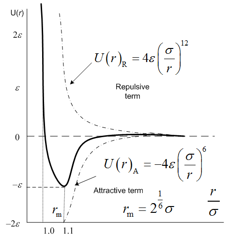 | Figure 1. Lennard-Jones potential |
The Lennard-Jones potential is used to describe the interactions in simple fluid such as noble gas argon.
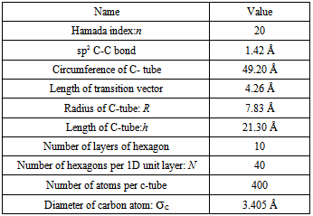
3. Structure of Carbon Nano Tube
Because three carbon nano tubes are chosen as solid phase in canonical ensemble, it is necessary to study its structure as follows.A nanotube is formed by rolling a graphene sheet (rectangle: ABB’A’) into a cylinder. Its structure can be uniquely characterized by defining Hamada indices: n and m of the chiral vector ,which is shown as[15, 16](see Figure 2):  | (9) |
Where the vectors a and b are lattice vectors of a graphene sheet. They have 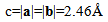 On the basis of equation(9), it is able to generate three basic types of nano tubes. The shape of the graphene sheet at the end of the tube is named as follows according to the values assigned to n and m:1. "armchair", where n = m, 2. "zig-zag", where m = 0, 3. "chiral", with any other combination of n and m.
  | Figure 2. Zig-Zag carbon nano tube |
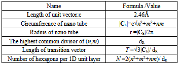
T and h in Figure 2 are called transition vector and length of tube respectively. Some concerned parameters and formulas to build a carbon nano tube are listed in Table 1.Table 1. some formula used for generating carbon nano tube
 |
| |
|
4. Methodology
In this research, modelling is performed in canonical ensemble. Three same size “zig-zag” carbon nano tubes are built and located into the cubic box V and filled with fluid particles to form a heterogeneous phase system with constant number of fluid particles (N) and temperature (T).
4.1. Mathematical Expression of Geometric Properties for Cubic Box and Carbon Nano Tubes in Canonical Ensemble
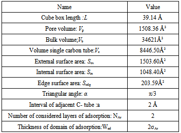
Some parameters and spatial location of three nano tubes in cubic lattice are presented in Figure 3. 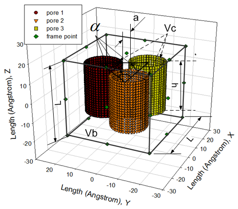 | Figure 3. three carbon nano tubes in the cubic box to form canonical ensemble |
The temperature and number of particle fluid are easily confirmed by input. However, the length of cubic box is decided after length of carbon nano tubes is built to ensure them be located in the centre of box. In this project, three carbon nano tubes are built in zig-zag style, hence n=20 and m=0. Some physical properties of them are shown in Table 2.Other extended physical properties are also generated and listed in Table 3 respectively.Table 2. some physical properties of zig-zag carbon nano tube
 |
| |
|
The radius of carbon nano tube R calculated by the formula supplied in Table 1did not specify internal or external radius of the tube. However, there is a thickness for a carbon nano tube wall. In order to effectively consider how adsorption, R is regarded as an inner radius of carbon nano tube. Therefore, the pore volume Vp which is used to calculate volume density of particles remaining inside pores on average is expressed as | (10) |
Correspondingly, the volume of single carbon nano tube is calculated by considering the thickness of its wall: | (11) |
The bulk volume Vb is the space minus three volumes of carbon nano tubes in the box. Thus | (12) |
Where the volume of cubic box V is obtained by  | (13) |
It is easy to calculate the surface area of internal and external tubes and the one of their edges at top and bottom by following equations:Internal surface Sin | (14) |
External surface Sext | (15) |
The surface area of top and bottom Sedg | (16) |
The value of above parameters is shown in Table 3 respectively.Table 3. physical properties of cubic box and extended physical properties of zig-zag carbon nano tube
 |
| |
|
4.2. A Special Technique Used in Distributing Fluid Particles in Cubic Box and Configuration of System
Compare with simulation of pure fluid particles in homogeneous phase system, modelling in fluid particles interacting with solid phase in canonical ensemble is extremely difficult.The most difficult is how to distribute fluid particles in spatial space existing solid phase. The traditional manner in deal with distributing fluid particles is using lattice box. However, as shown in Figure 3, the spatial positions occupied by carbon atoms in cubic box are not allowed to accept fluid particles. In other words, fluid particles are only able to be distributed in the rest spatial space. However, the rest part of it is a typically irregular geometric shape. In order to overcome this difficulty, author design a special algorithm for it. The principle is that If fluid particles do not touch the three carbon nano tubes, they can go someplace else until the rest spatial space is filled. In short, do not touch, go someplace else.The mathematical expression above principal is as follows, | (17) |
A very small value can be selected as a tolerance. F and C represent a spatial point in a given Cartesian coordinates system, thus in the cubic box respectively. In this case, F can represent a set of spatial points of fluid particles, and C represents a set of spatial points of carbon atoms located in carbon nano tubes in cubic box respectively. Any spatial distances between two spatial points thus F−C must be larger than or equal to an arbitrarily given tolerance. In fact, F−C forms a distance vector field in the cubic box.Expression of Special Technique Using FORTRANBuild lattice in Cubic BoxOnce the length (height) of carbon nano tubes h is confirmed, the size of cubic box Boxlength L is also determined by assuming: | (18) |
to make sure three carbon nano tubes inside the cubic box.What should do at the next step is to lattice the cubic box so that the fluid particles are able to be distributed into it. At this stage, the spatial structure and position of three carbon nano tubes are unnecessary to be considered. The focus is only located on creating lattice in the cubic box and then distributing fluid particles into it. The code of SUBROUTINE INI_PAR_LATTICE using FORTRAN 90 in Figure 4 shows how to lattice the cubic box. 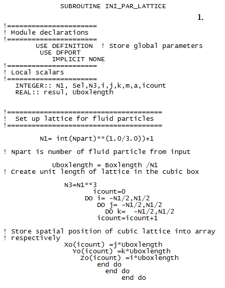 | Figure 4. create unit length of lattice in cubic box with FORTRAN 90 |
The unit length of lattice Uboxlength is an important parameter in building lattice inside the cubic box (see Figure 3). To obtain it, at first, assume that the cubic box is fully filled by fluid particles whose number is determined by input NPART, thus constant number of fluid particles N. Then, the number of spatial points in one-dimensional direction N1 appearing in the cubic box can be easily obtained by  | (19) |
Then total number of spatial points in three-dimensional lattice N3 inside the cubic box is simply expressed as | (20) |
Also, the unit length of lattice is isotropic, accordingly the unit length of lattice Uboxlength is calculated by  | (21) |
Now it is easy to build the lattice using three-dimensional loop. In order to distribute initial spatial position of fluid particles around three carbon nano tubes being located in the centre of the cubic box, the spatial position of fluid particles is taken into account from –N1/2 to N1/2.The location of spatial points are then stored into corresponding array in x, y and z direction respectively. Each array is indexed by a unique index icount. Create a Condition to Distribute Fluid Particles in Cubic Box Containing Solid PhaseAfter building the lattice in cubic box, the next step is to distribute fluid particles. In the homogenous phase system, distributing fluid particles is easily performed. As pointed out it above, it is extremely difficult to distribute them into an irregular spatial space in the cubic box due to solid phase existence. Although the simple rule of “do not touch, go someplace else” is already proposed by author, how to carry out it in computer practice is a vital procedure. In order to implement it, author designed simple codes in FORTRAN 90 (see Figure 5). In these codes, it emphasises that the spatial position of each fluid particle must be compared with the one of each carbon atom locating three nano tubes in terms of calculating spatial distance before it is located into one spatial position at one point of lattice. The following points should be noticed when read these codes.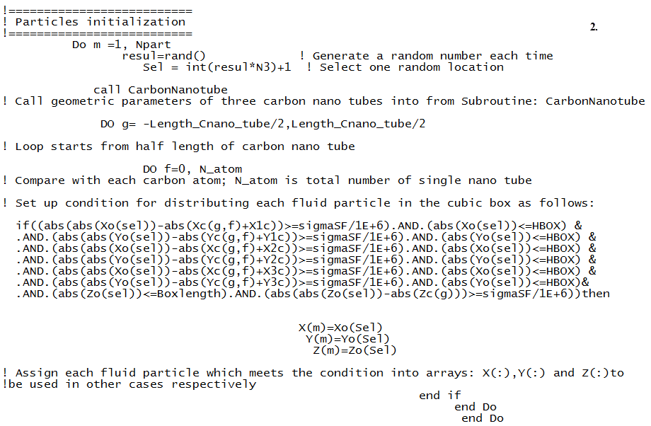 | Figure 5. set up condition to compare spatial position of each fluid particle with the one of carbon atom in three carbon nano tubes with FORTRAN 90 |
1. HBOX is half length of cubic box, its value is equal to Boxlength/2; 2. sigmaSF/1E+6 is very small value as a arbitrary tolerance;3. Xc(:,:), Yc(:,:) and Zc(:,:) are two-element arrays in x,y and z direction to form spatial structure of three nano tubes in the cubic box system (see Figure 3);4. X1c, X2c,…, Y3c, Zc is spatial location of three nano tubes in the cubic box system(see Figure 3);5. Because spatial position of cubic lattice is located into eight sections with positive and negative sign in a cubic box based coordinates system, the built-in function abs() is then used to ensure obtained value is always larger than or equal to an positive arbitrarily given tolerance;6. Using 'ABS(A-B)>= one VALUE' instead of 'A/=B' to represent the unequal between A and B, in other words there is a distance between A and B, thus “do not touch”. A and B can be a numerical value generated by corresponding spatial point in the lattice respectively;7. Using 'ABS(A-B)<= one VALUE' instead of 'A==B' to represent the equal between A and B or the inclusive between them. Otherwise, the designed condition could never be met in the calculation. The supplied codes play a vital role in this research. It does not need to consider a complicated geometric problem when initializing spatial position of fluid particles in the cubic box. On the other hand, another significant is that it converts three-dimensional calculation to be one-dimensional calculation and judgment (Yes or No), thus following up one-dimensional direction to compare one-dimensional spatial point with the one determined by two dimension. Therefore, a large number of CPU time is saved.Remove Filled Spatial Position and Control Process of Distributing Fluid Particles During distributing fluid particles, another topic which have to be considered is that once one spatial position is successfully is occupied, this occupied spatial position must not be considered when other fluid particle is randomly selected at next time.The supplied codes in Figure 6 provide a trick to effectively handle it. When above comparison is performed each time, the process of reducing spatial space can be achieved by increasing index a in each given array, in which the index is already assigned into the existing arrays and then assigning them into the current arrays respectively. On the other hand, number of fluid particles is also reduced at the same time so that running is to be automatically terminated when it equals to zero. Therefore, how much spatial space (or spatial points at lattice) is available to be used or occupied, which is simultaneously influenced and controlled by above two procedures. Once the number of distributed fluid particles reaches to zero (thus N3==0), the process of distributing fluid particles in cubic box is terminated.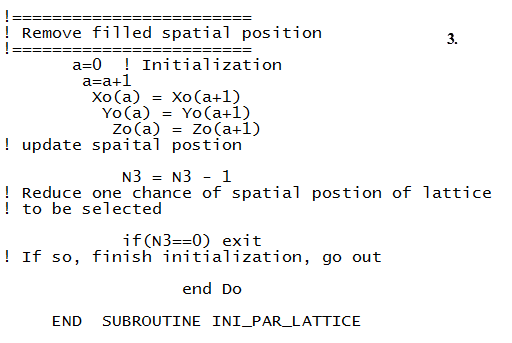 | Figure 6. remove filled spatial position in cubic box with FORTRAN 90 |
Results of Initializing Fluid Particles in Cubic Box Figure7 demonstrates the process of distributing fluid particles in the cubic box without touching the walls of three carbon nano tubes. As seen from Figure7, the rest available spatial space is being decreased while the number of fluid particles entering cubic box is increasing. Once the inputted number of fluid particles is reached to, the process of initializing fluid particles is terminate immediately. However, there is still a spatial space to be available. It is easy to estimate density of fluid particles by means of combining the number of fluid particles and the available volume calculated by equation (11)−(13). In practice, this functionality feature is very useful to create high density fluid or dilute gas for one selected ensemble to investigating the physicochemical properties happening in either homogenous or heterogeneous system.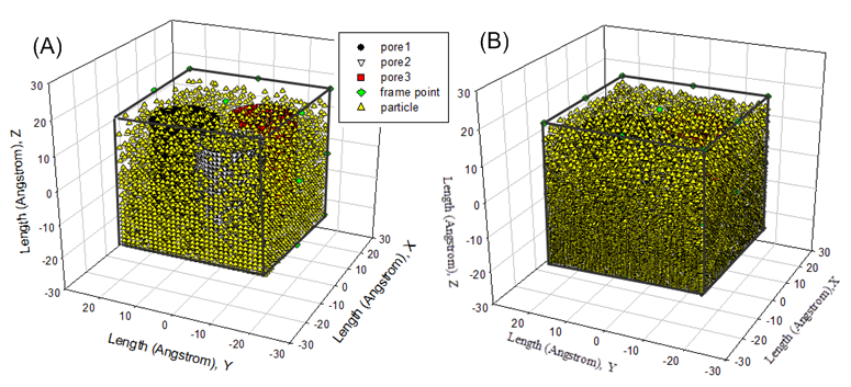 | Figure 7. (A) initial distribution of 18000 fluid particles ; (B) initial distribution of 25000 fluid particles in cubic box containing three carbon nano tubes |
Above process is quickly achieved, however it requires extra physical memory to continently and effectively support post-process such as plotting figures when the number of fluid particles is large enough.Application in Configuration of SystemActually, the above proposed principle as a condition of controlling fluid particles can be applied into not only updating configuration of system of fluid particles if their trial movements are successful but also tracing trajectory of fluid particles. As mentioned in the preceding section, If each randomly selected particle’s trial fails, the original spatial position (xo,yo,zo) is still assigned to it; otherwise the new spatial position (xn,yn,zn) is assigned to it. The new spatial position for each fluid particle is confined by two conditions:1. It must be inside the cubic box to keep a constant number of fluid particles. 2. It is allowed to touch the wall but cannot occupy the spatial position of wall. To satisfy the first and second condition, it can be easily achieved by designing the following algorithm.For fluid particles in the bulk, for example, If xn> HBOX, then xn= HBOX - (HBOX/50.0)Similarly,If yn> HBOX, then yn= HBOX - (HBOX/50.0)And If zn> HBOX, then zn= HBOX - (HBOX/50.0)However, for fluid particles moving inside cubic box after successful trials, the condition shown in Figure 5 is useful in determining new spatial position for each fluid particle. Therefore, inequality(17) as a general rule is very useful in checking the new spatial position for each fluid particle when the configuration of system takes place each time.This principle likely has an analogy to the correlation(4). However, the difference is that the criterion of the correlation (4) is based on Boltzmann factor, thus the difference of potential energy rather than spatial distances shown by inequality(17).
4.3. Design a Domain for Adsorption and Desorption
Because the absorption and desorption of molecules imposing upon the wall and edge take place simultaneously, to describe this process, it is necessary to design a domain and boundary of a film to consider it. The thickness of domain is arbitrary. In this case, imagine that there is a film locating outside wall and edge with the thickness Wad = 2σAr. The fluid particles flow into and out of this film (see Figure 8).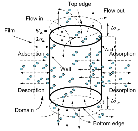 | Figure 8. design domain of adsorption and desorption |
Whether fluid particles remaining inside the designed domain or moving outside it is based on spatial distance between spatial position of each designed domain and the one of fluid particles.Some fluid particles may be already located into designed domains when they are initially distributed into the lattice of cubic box. However, for Monte Carlo simulation, the concerned topic is its final approach under the condition supplied by the selected ensemble. Designing an arbitrary domain is for easily observing fluid particles’ behaviour during each cycle is performed. Naturally, so-called adsorption and desorption between solid-fluid phase simultaneously happen in the process of fluid particles moving into or out of the designed domains. Some basic techniques introduced above are still useful in this approach.Procedure of Modeling Adsorption with Monte Carlo in Canonical Ensemble Containing Heterogeneous System.In the preceding section, some theoretical concepts and main relevant techniques applied into this research are already introduced. However, Monte Carlo method based modelling heterogeneous phase system is a very complicated process. In order to know how whole procedures are implemented, briefly describing them is presented in Figure 9. Monte Carlo simulation is also interpreted as a process of Markov process. The probability of fluid particles’ trials with condition and corresponding distribution dynamically varies in one given three-dimensional matrix (lattice). The energy variation of fluid-fluid and fluid-solid in heterogeneous system is updated with respect to spatial distance change. The energy variation becomes a condition assessed by Boltzmann factor to describe a process of each trial of fluid particle and determine its success or failure probability from one state (cycle) to another. The process of variation of system is then called as configuration of system. Depending on what wants to approach and be obtained, in this case, some specific designing is used for investigating argon adsorption and desorption onto walls of three nano tubes. Therefore the program consists of many subroutines to achieve the target.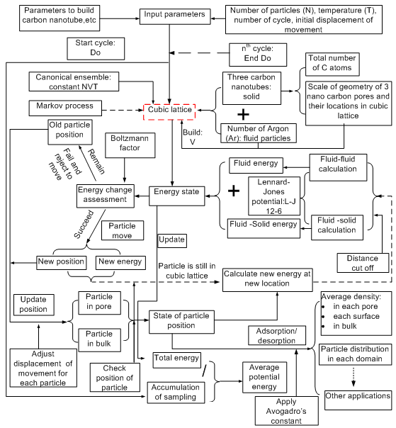 | Figure 9. schematic procedure of modeling Ar adsorption in canonical ensemble comprising of three carbon nano tubes with Monte Carlo method |
However, the focus in this paper restricts within the range of introducing one key technique used in modelling heterogeneous phase system.
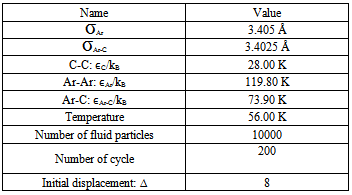
4.4. Some Physical Properties of Argon Fluid Particle and Carbon Atom
When applying equation (8) into calculating potential pairwise particles, the combined parameters: σAB and εAB need to estimate if the subscript A and B represent different fine particles such as molecule and atom. The following useful formulas thus the Lorentz-Betherlot rule[14]can be used to assess the coupled properties of them. | (22) |
 | (23) |
The values of the Lennard-Jones potential parameters are listed in Table 4.Table 4. some physical properties of fluid particle and carbon atom
 |
| |
|
5. Results and Analysis
5.1. Fluid Particle Distribution in Cubic Box
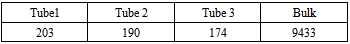
Initial DistributionArgon is treated as fluid particles in a canonical ensemble when Monte Carlo simulation is performed.The initial state of them with three carbon nano tubes is presented in Figure 11(A). As seen from it, following the principle: “don’t touch, go someplace else”, the fluid particles are randomly distributed in the cubic box without touching three tubes. In this case, 10000 particles are mainly located into space occupied by the bottom parts of three tubes. Some particles are distributed into space at the top of three tubes and three pores (see Table 5).Table 5. number of particles in an initial state
 |
| |
|
Visualize Particle Distribution When RunningAfter initialize the particles in cubic box, the first attempt of each particle is based on initial displacement ∆, which is to be updated randomly accompanying with variation of system. The number of particles distributing in different domain at running time is shown in Figure 10. 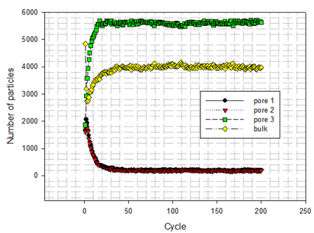 | Figure 10. numbers of fluid particles distributing in different domain at running time |
There are three examples (see Figure 11 (B), Figure 12(A) and (B)) to describe how fluid particles are distributed when particles locating in different domains as indicated by Figure 8 carry out each trial. As discovered from them, the configuration of fluid particles in the canonical ensemble is dynamically updated when some trials of fluid particles are accepted or rejected.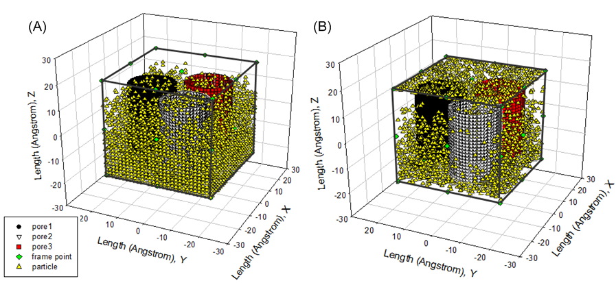 | Figure 11. (A) initial fluid particles distribution; (B) fluid particles distribution at 3rd cycle |
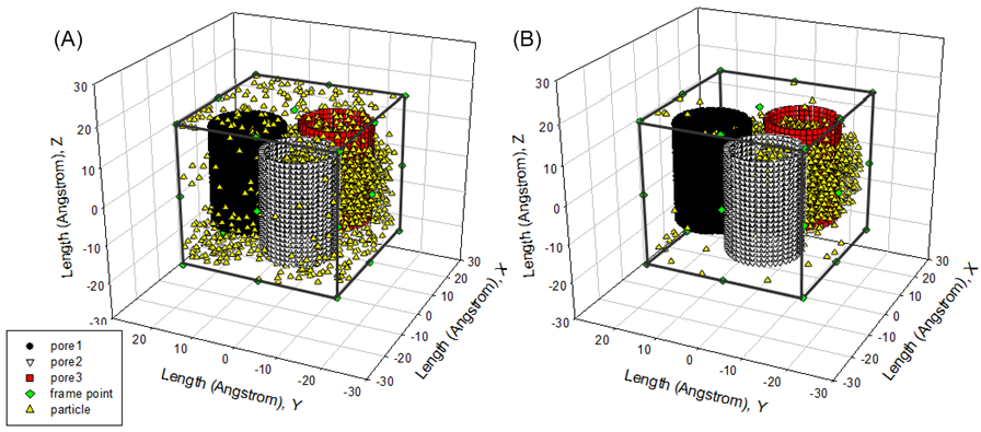 | Figure 12. (A) fluid particles distribution at 11th cycle; (B) fluid particles distribution at 19th cycle |
5.2. Physical Properties of Fluid Particles
Successful Trial As seen from above, fluid particles move at all time in the given canonical ensemble. Movement of fluid particles are not only captured in the bulk (see Figure 11(B), Figure 12 (A) and (B)) but also represented inside pores (see Figure 13). Of interest is that fluid particles have the tendency to move to the centre of three nana tubes at initial cycles. However, such temporary state is updated in the rest cycles according to the distribution of number of fluid particles shown in Figure 10.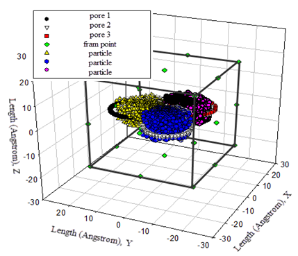 | Figure 13. fluid particles are located inside pore at the 6th cycle |
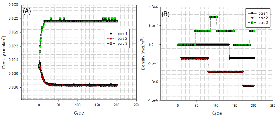
In order to illustrate how adsorption and desorption occur in each domain illustrated by Figure 8 , based on the known size of geometry given in Table 3 some physical properties are presented in Figure 14 (B) − Figure 16(B) after running. Fluid particles appear in different domains and configuration of system is updated repeatedly. The number of fluid particles is then converted into mole per cubic meter and square area using Avogadro’s constant (6.02214×10²³ molecules/g-mol).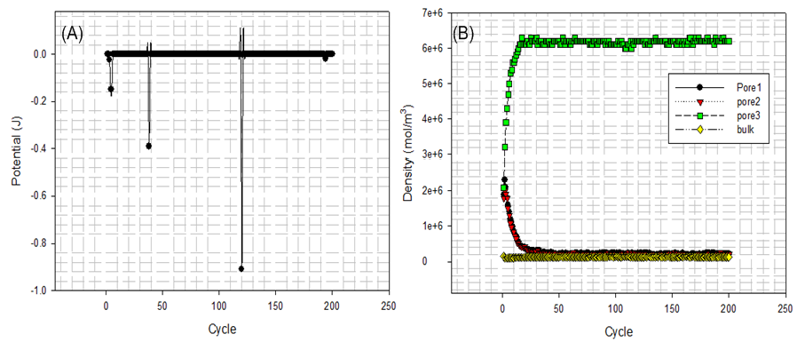 | Figure 14. (A) overall potential energy changes; (B) densities of fluid particles in pores and bulk |
 | Figure 15. (A) fluid particles enter and leave domain at inner surface; (B) fluid particles enter and leave domain at external surface |
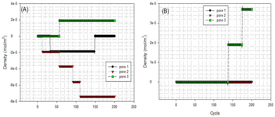 | Figure 16. (A) fluid particles enter and leave domain at bottom surface edge; (B) fluid particles enter and leave domain at top surface edge |
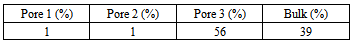
At first, Figure 14 (A) shows that how average potential energy of system waves when the configuration of system is frequently updated. In this case, the attractive term shown by equation(8) plays a main role in driving fluid particles to move. Figure 14(B) shows that how much amount of particles actually existing in three different pores and bulk per unit cubic meter on average during running. Similarly, Figure 15 and Figure 16 provide some information of how fluid particle leaves and enters designed domains per unit square meter.Combining the results of Figure 10 and Figure 14 (B) with the one of Figure 15(A), it can be discovered that a number of fluid particles quickly leave pore 1 and 2 at several initial cycles. In opposition to them, the number of fluid particles in pore 3 increases. The increased number of fluid particles in pore 3 does not mean all particles inside it come from the pore 1, 2. Some of them come from bulk. At the same time, adsorption and desorption take place at external surface areas and the ones locating at both side edges in terms of Figure 15(B) and Figure 16 (A) and (B). The positive value represents that fluid particles enter the domain thus adsorption. Inversely, the negative means that fluid particles leave that domain thus desorption. It should be pointed out that some fluid particles already exist in some designed domains when they are distributed initially and randomly (see Figure 11(A)). Consequently, once fluid particles are activated by assigning an initial displacement ∆ which is to be updated randomly and atomically in each cycle, the movement of them starts within whole heterogeneous system accompanying with adsorption and desorption occurring in designed domains immediately.On the other hand, as visualized from Figure 11(B), Figure 12(A) and (B), an amount of fluid particles is absorbed by the external surface area of tube 3. And less fluid particles appear on the external surface area of pore 1 and 2. Another concerned topic is that how fluid particles flow in and out the pores. When the diffusion of fluid particles happens, fluid particles are very sensitive to the interaction with carbon atoms locating at exits of three tubes. If the more fluid particles appear at surface area of edges at top and bottom, it means the more chances for fluid particles to flow into or out of that pore. As expected, on the basis of Figure 14(B), Figure 15 (A) and Figure 16(A) and (B), the more fluid particles flow in and out from both exits of pore 3. Such behaviour approaches to a constant, thus the balance of flowing in and out reaches to a state of dynamic equilibrium finally because most fluid particles approach to being located inside and outside pore 3.The final result listed in Table 6 clearly shows that 56% of fluid particles are remained in the pore 3 when the final cycle is reached to. Therefore, fluid particles are unevenly distributed in different domains. Most fluid particles move to and are located at the spatial place where most fluid particles already existed because the spatial distance amongst them (fluid-fluid, fluid-solid) is shortest according to L-J potential equation(8).Table 6. final percentage of fluid particles distributed in domains
 |
| |
|
Unsuccessful Trial In above section, the successful trials are recorded into different domains. The configuration of system is updated by each trial of fluid particles. It is discovered that most trial of particles are successful. However, unsuccessful trials are also recorded and listed in Table 7. Because of that, the particles are remained in the original state indicated by coordinates (x, y, and z) in Table 7.Table 7. unsuccessful trial of fluid particles
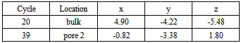 |
| |
|
It is worth pointing out that all information (data) about the spatial position of fluid particles when they move in the cubic box are stored into array X (:), Y (:) and Z (:) as codes are shown in Figure 5 no matter whether each trial of fluid particle is success or failure as long as the geometric conditions for specific domains are designed. It is easy to store and retrieve data from them to display corresponding figures.
6. Conclusions
In this research, a new manner in dealing with heterogeneous system has been proposed. Its new features are surmised as follows:1. Following the basic principle of “do not touch (solid phase), go someplace else”, the fluid particles are quickly distributed in cubic box. The dimension is dramatically reduced to one dimensional comparison; therefore a lot of CPU time is saved. Such a principle is also applied into any fluid-solid phase modellings.2. The novel expression of adsorption and desorption is accordingly generated on the basis of number of fluid particles entering into or moving out of specific domain.3. It is easily to visualize the trace of fluid particles and record all successful trails and unsuccessful trials in the canonical ensemble.4. In this case study of canonical ensemble, it is discovered that fluid particles locating in three pores have a tendency to move to the centre of three tubes. That is because the distance of fluid particles and carbon atoms is shortest. The attractive term in Lennard-Jones potential play a main role in this tendency. 5. Because number of fluid particles in pore 3 is larger than the one existing in other pores, it can be discovered that a certain amount of fluid particles is adsorbed onto its external surface.
ACKNOWLEDGEMENTS
Author addresses special thanks to Professor Peter Halley at school of chemical engineering, University of Queens land for his support.
References
| [1] | C. Fan, D. D. Do, D. Nicholson, J. Jagiello, J. Kenvin, and M. Puzan, "Monte Carlo simulation and experimental studies on the low temperature characterization of nitrogen adsorption on graphite," Carbon, vol. 52, pp. 158-170. |
| [2] | J. Cheng, L. Zhang, R. Ding, Z. Ding, X. Wang, and Z. Wang, "Grand canonical Monte Carlo simulation of hydrogen physisorption in single-walled boron nitride nanotubes," International Journal of Hydrogen Energy, vol. 32, pp. 3402-3405, 2007. |
| [3] | S. Bandyopadhyay and S. Yashonath, "A Monte Carlo Method for Estimation of Pore Volumes of Zeolites," Zeolites, vol. 19, pp. 51-56, 1997. |
| [4] | P. Bai and J. I. Siepmann, "Selective adsorption from dilute solutions: Gibbs ensemble Monte Carlo simulations," Fluid Phase Equilibria, vol. 351, pp. 1-6. |
| [5] | K. G. Ayappa, "Influence of temperature on mixture adsorption in carbon nanotubes: a grand canonical Monte Carlo study," Chemical Physics Letters, vol. 282, pp. 59-63, 1998. |
| [6] | G. C. Boulougouris, L. D. Peristeras, I. G. Economou, and D. N. Theodorou, "Predicting fluid phase equilibrium via histogram reweighting with Gibbs ensemble Monte Carlo simulations," The Journal of Supercritical Fluids, vol. 55, pp. 503-509. |
| [7] | C. Fan, D. D. Do, and D. Nicholson, "Bin-Monte Carlo simulation of ethylene coexistence and of ethylene adsorption on graphite," Colloids and Surfaces A: Physicochemical and Engineering Aspects, vol. 437, pp. 42-55. |
| [8] | L. Firlej, B. Kuchta, A. Lazarewicz, and P. Pfeifer, "Increased H2 gravimetric storage capacity in truncated carbon slit pores modeled by Grand Canonical Monte Carlo," Carbon, vol. 53, pp. 208-215. |
| [9] | M. Rahmati and H. Modarress, "Nitrogen adsorption on nanoporous zeolites studied by Grand Canonical Monte Carlo simulation," Journal of Molecular Structure: THEOCHEM, vol. 901, pp. 110-116, 2009. |
| [10] | T. J. B. Bandosz, Mark James Gubbins, Keith E.Hattori, Y. Iiyama, T. Kaneko, Katsumi Pikunic, Jorge Thomson, Kendell T., Molecular Models of Porous Carbons, Ljubisa R. Radovic ed. vol. 28: Marcel Dekker Inc, 2003. |
| [11] | V.I.Kalikmanov, Statistical Physics Basic concepts and applications. Berlin Heideberg: Springer-Verlag, 2001. |
| [12] | B. S. Daan Frenkel, Understanding Molecular Simulation From Algorithms to Applications. San Diego: Academic Press, Inc., 1996. |
| [13] | D. Chandler, Introduction to modern statistical mechanics. New York: Oxford University Press, Inc, 1987. |
| [14] | R. B. B. W. E. S. E. N. Lightfoot, Transport Phenomena. New York: John Wiley & Sons, Inc., 2002. |
| [15] | C. T. S. Reich, J. Maultzsch, Carbon Nanotubes Basic Concepts and Physical Properties. Wcinhcim: WILEY-VCH Verlag GmbH & Co. KGaA, 2004. |
| [16] | G. D. M. S. DRESSELHAUS, R. SAITO, " Physics of carbon nanotubes " Carbon, vol. 33, pp. 883-891, 1995. |
 Abstract
 Reference
 Full-Text PDF
 Full-text HTML