1. Introduction

The volatility of food product prices since the food crisis of 2007/2008 is one of the priority problems to which agricultural policies have tried to respond in recent years. This attention is due to their short-term impact on the purchasing power of consumers. Still, also in the long term the incentive for producers to produce more [1] and consequently budgetary imbalance arises. Consumers fear an increase in the cost of access to food products, while producers fear a drastic drop in their income. In either case, the effects of the disturbances reinforce precariousness and weaken the actors to the point of forcing policymakers to take measures to reduce price uncertainty in agricultural markets, since more people can’t afford a healthy diet because of a high price.

Given its wealth of human and raw material resources, its expertise, and a vast market, the African continent has immense potential, which should enable it not only to feed itself, to eliminate hunger and food insecurity, but also to become a major player in international markets. However, Africa is the continent that harbors a high rate of malnourished people [2] with a rate of 19.1% of undernourished people (which is more than double the world average of 8.9% in 2019) against 17.6% in 2014, that is to say that in 10 undernourished people in the world, 4 are African, and one in four Africans suffer from undernourishment [3,4]. Within families, young children, as well as pregnant and lactating women, are the most affected and even more susceptible to nutritional deficiencies [5]. Undernutrition for pregnant and lactating women has direct effects on foetuses because undernutrition during the foetal period and the first months of life contributes to both immediate and long-term health problems. It should be noted that child malnutrition can permanently affect the intellectual (lower IQ) and physical abilities (developing chronic diseases in adulthood, including obesity and diabetes) and jeopardize the future of entire sections of the population [5,6].

Sub-Saharan Africa is particularly concerned by this burden of undernourishment because it is the region that, in addition to the galloping demography, is home to a high number of people suffering from hunger, with a rate of 22%. In this region of Africa, the East African Community (EAC) is the second after Central Africa to experience the highest rate of undernourishment in 2019 (27.2%) [8]. The report by [7] highlights that in terms of numbers and outlook, all other things being equal, with the trends observed over the past decade, the world and in particular Africa and even more East Africa is by far able to meet the daunting challenge of achieving the "Zero Hunger" objective of the 2030 Agenda of the Sustainable Development Goals (SDGs). It is estimated that the rate of undernourished people in 2030 will be 33.6% in East Africa without considering the impact of the COVID-19 pandemic.

To eradicate this food insecurity, which has long shaken the continent, African Heads of State have drawn up strategic documents and set themselves objectives putting Agriculture and the Farmer at the center of development, which is obvious for a continent. With an agricultural vocation to 48% of the population (70% for East Africa) and whose GDP relies heavily on agriculture [5]. In this section, the EAC has had an agricultural and rural development policy since 2006. It adopted an action plan on food security in 2011, aligned with the priorities of the Detailed Plan for the Development of Agriculture in Africa (DPDAA)¹[5]. These policies allowed for an increase in production, but productivity remained a continental desire.

Despite the combined efforts of these policies, which have allowed an increase in production in general, except in recent years when production has fallen following climatic disturbances, the El Niño phenomena, and the locusts that have recently devastated crops, agricultural prices maintained an upward trend in volatility, thus leading to a decline in household purchasing power and implicitly to a loss in the value of local currencies.

This paper will show the impact of food price volatility on the production and utilization of agricultural products, particularly rice and corn products, which constitute the staple diet in the EAC block and occupy a significant share of the caloric intake in the diet [9].

2. Literature Review

2.1. Agricultural Landscape in the East African Community (EAC)

The East African Community (EAC) is fundamentally an agriculture-driven region. Despite this, agricultural production and productivity levels remain below global benchmarks [10]. Farmers across the EAC face substantial obstacles in boosting output and efficiency, stemming from a complex interplay of political, natural, and technological factors. Specifically, policy shortcomings include inadequate legal and regulatory frameworks, coupled with weak institutional support. Natural factors limiting productivity encompass natural resource degradation and the increasing pressures of climate change. Technologically, the region suffers from limited adoption of yield-enhancing inputs, such as improved seed varieties, fertilizers, appropriate animal fodder and feed, critical veterinary vaccines, and modern agricultural equipment and machinery. These constraints collectively contribute to, and exacerbate, poor farm management practices across the region. The majority of farmers in the EAC operate as small-scale subsistence farmers, cultivating small landholdings [10,11]. This demographic faces numerous challenges, including limited access to crucial financial resources needed to purchase yield-improving inputs, alongside the inherent instability of agricultural commodity prices in local markets. Broader, cross-cutting issues that negatively impact agricultural production include pervasive poverty, gender inequality, and the under-representation and engagement of youth in agricultural activities. Addressing the multifaceted nature of these challenges requires a comprehensive strategy that promotes more resilient and sustainable agricultural production systems across the EAC.

2.2. Food Price Volatility in the EAC Sub-Region

Food price volatility has been a persistent and significant problem in Eastern Africa for decades. Recurrent surges in food prices have severely impacted food security and the livelihoods of vulnerable populations throughout the region [9,10]. The global food price crisis of 2008–2009 stands out as a particularly impactful event. This crisis was fueled by several converging factors, including escalating food demand from rapidly developing economies like China and India [14], adverse weather patterns in key agricultural producing nations [15], and the global financial crisis, which drove increased speculative investment in food commodities, as well as increases in energy and fertilizer costs [16]. The consequences were dire, leading to a deepening of hunger and poverty across Eastern Africa. Millions were unable to afford adequate and nutritious food, forcing many to adopt detrimental coping mechanisms, such as selling essential productive assets or incurring debt simply to survive [16,17,2]. This crisis underscored the vulnerability of the region to external economic shocks and highlighted the urgent need for developing more resilient food systems capable of withstanding such pressures. Following the 2008-2009 crisis, the Consumer Price Index (CPI) in East African nations has demonstrated fluctuations, yet generally exhibits an upward trend, mirroring persistent inflationary pressures within food markets [19]. Other significant food price spikes occurred in the region in 2011, 2012, and 2017, each driven by a combination of regional droughts, global commodity price fluctuations, and domestic economic factors such as currency depreciation and instances of conflict [19,20]. These repeated and disruptive shocks have placed significant strain on household budgets and have undermined food security for millions of people living within the region [6,21]. East African nations have experienced significant changes in their Consumer Price Index (CPI) over the past decade, impacting the affordability of necessities and overall economic stability. Furthermore, food price volatility presents a persistent challenge to food security and nutrition in the region.

2.3. CPI Trends in East Africa

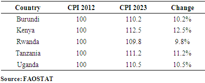
Table 1 illustrates the evolution of CPI in the East African Community (EAC) between 2012 and 2023. Data, sourced from FAOSTAT, reveals a consistent upward trend across all member states.

Table 1. Evolution of CPI in EAC during the last decade

As evident in Table 1, Kenya experienced the largest CPI increase at 12.5%, while Rwanda saw the smallest rise at 9.8%. This increase in CPI has several significant impacts. It reduces the purchasing power of incomes, making it more difficult for individuals and families to afford essential goods and services such as food, shelter, and clothing. Beyond the general impact on well-being, food price volatility, linked to CPI increase, poses a direct threat to food security and nutrition in East Africa. Rising food prices can force vulnerable populations to reduce their food consumption, leading to malnutrition and associated health problems. It can also contribute to social unrest and political instability. Despite these challenges, East African countries have demonstrated economic growth, resulting in positive developments like poverty reduction and improved living standards. However, mitigating the negative effects of CPI increases and food price volatility remains crucial for sustained and inclusive development.

2.4. Understanding Price Volatility

Price volatility is a statistical measure of the fluctuations in the price of an asset over a specified period. It is often quantified using the standard deviation of returns, indicating the extent to which returns deviate from their average. Engle [4] succinctly describes volatility as a consequence of the arrival of new information in the market. More broadly, volatility represents the degree of variability in prices or quantities [23] or the fluctuation of prices around the long-term equilibrium or trend [23,24]. As Previdoli [26] argues, the value of a financial asset hinges on the future gains investors anticipate. In the context of agricultural businesses, White & Dawnson [27] highlight the importance of expected harvest prices in planting decisions. While increasing prices can incentivize production and increase profits [26,27], such income is inherently uncertain, and dependent on future economic conditions. Investors rely on real-time information to forecast fair asset prices, and the arrival of new information necessitates revisions to these forecasts, leading to price fluctuations. Volatility, therefore, provides critical information about the uncertainty and risk associated with investments. High volatility implies the potential for significant price swings in a short period [26]. An investor's risk tolerance and desired return will influence their willingness to accept high volatility.

Two key types of volatility are distinguished:

• Historical (ex-post) or unconditional volatility: This measures the realized variability of prices over a long period, assuming constant variance [25,23,32,33,34]. It allows for the measurement of the dispersion of values compared to the average.

• Conditional (dynamic) or ex-ante volatility: This refers to forecasting future market volatility based on currently available information. The literature widely acknowledges that price series for economic goods, including agricultural prices, often exhibit trends and seasonality [23]. Therefore, econometric analyses are needed to account for the time-varying nature of variance [36]. ARCH and GARCH family models, as well as nonparametric models, fall into this category.

Understanding and managing both CPI increases and food price volatility are vital for ensuring food security and promoting sustainable economic development in East Africa. Further research and policy interventions are needed to mitigate the negative impacts of these factors and build resilience within the region's agricultural systems and economies.

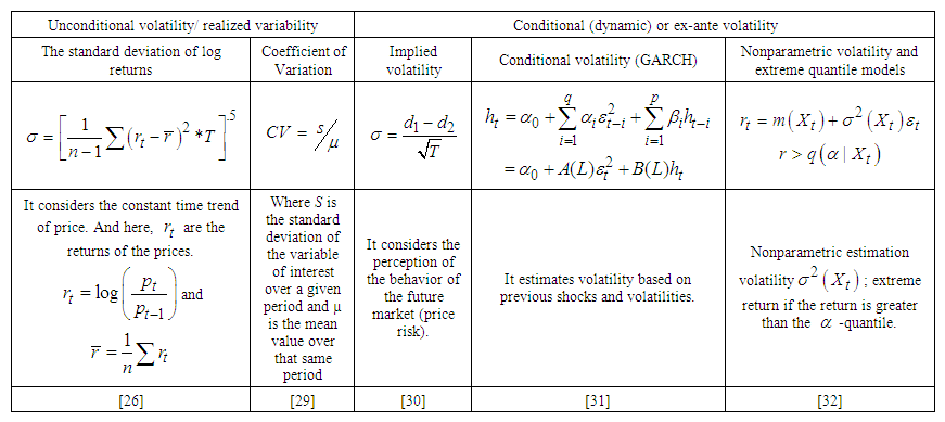Table 2. Different measures of volatility

3. Research Methodology

The study focused on the EAC member countries, and due to the irregularity of the data for South Sudan and Uganda, only the four former member countries of this community were considered: Burundi, Kenya, Rwanda, and Tanzania.

3.1. Source and Nature of Data

Existing databases from international institutions responsible for statistics, such as the World Bank and FAOSTAT, served as data sources. This study spans 53 years (from 1966 to 2018) for the food availability model and 19 years, from 2000 to 2018, for the food utilization model due to missing data on certain variables over a longer period. We used Excel, Stata, and/or EViews software for data collection, entry, processing, and analysis.

3.2. Definition of Variables

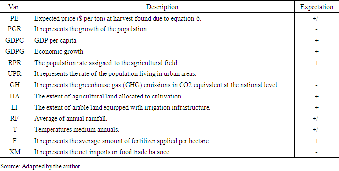
3.2.1. Food Availability Model

The volume of agricultural production is used as an indicator of food availability.

In equation 1, we focus on the effects of the volatility of producer prices represented by on the volume of agricultural production at the national level . This volatility is found using equation 7.

The control variables and determinants of production considered in the model are defined in Table 3:

Table 3. Definitions of variables in the food availability model

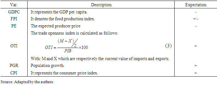
3.2.2. Food Utilization Model

To characterize the influence of price volatility on food utilization (food security pillar), the prevalence of anaemia in women of childbearing age (15-49 years) (dependent variable) was considered, which is a proxy of food utilization within families. The detailed equation is:

The meaning of the other control variables is presented in Table 4.

Table 4. Definition of the variables of the food utilization model

3.3. Analytical Framework

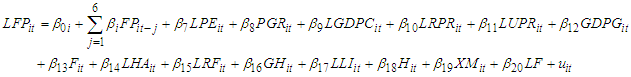
Multiple linear regression was used to characterize utilization and availability models. A GARCH(p,q) model (Generalized Autoregressive Conditional Heteroscedasticity), developed by Bollerslev [31] based on the ARCH model introduced by Engle [37], was used to estimate the volatility variable. The ARCH model allows the conditional variance to change over time, based on past errors, while keeping the unconditional variance constant [31]. The general estimating equation for the models is . denotes the total local production of a given good or the prevalence of anaemia among women of childbearing age and is the expected price while representing the predicted variance of the price, which measures volatility and the matrix of other explanatory variables. By assumption of linearity, an empirical specification of the availability model is the following:

(4)

With:

The GARCH process (p, q) is then used to generate the variables and . The price is a function of the information’s set of prices that are available at the moment and are given by:

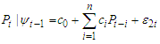(5)

is the expected average of the price, and under the assumption of homoscedasticity:

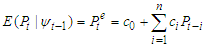(6)

The determination of the number of lags to consider is made using the information criteria in the EViews software. The errors in equation 5 are normally distributed with a mean of zero and variance :

(7)

And it is this last condition that defines the stationarity of the model [31]. The use of this model comes from the inspiration of the agricultural availability model established by Rezitis & Stavropoulos [38] and was extended by making a panel under the inspiration of the work of Lee [39]. Due to the subtlety of this model requiring short-frequency data, the annual data are transformed into quarterly frequency data following Denton's method using the EViews 10 software.

3.4. Model Diagnosis

3.4.1. Autocorrelation Test

According to Gujarati [40], the autocorrelation of errors is defined as the correlation between members of a series of observations ordered in time (time series data) or space (cross-sectional data) and it can result from several sources which are either the absence of an important explanatory variable or a bad specification of the model or either a smoothing by moving average or an interpolation of the data [41]. This problem is detected using several tests, but the most common is the Durbin and Watson (DW) test, which detects an autocorrelation of errors of the first order, and the Breusch-Godfrey test based on a Fisher test of nullity of coefficients or Lagrange multiplier "LM test", allowing to test an autocorrelation of an order greater than one and remains valid in the presence of the shifted dependent variable as an explanatory variable [40,41].

3.4.2. Homogeneity Test

The homogeneity test is based on the Analysis of Covariance (ANCOVA) of errors of cross-sections (individuals) and is based on a Fisher test [42]. It allows us to successively test three hypotheses:

1. The equality of all N slopes (parameter vectors) 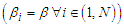and all model constants; which is called global homogeneity or homogeneous panel;

2. The N vectors of parameters are identical, while the constants are different depending on the individual . This case provides a panel structure with individual effects;

3. The N constants are identical, while the parameter vectors are different depending on the individual. In this case, only the constants among all the coefficients of the model are identical; we have therefore N different models.

4. Results of Econometric Analyses

4.1. Autocorrelation of Errors

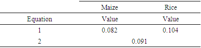
The DW test is used to assess the presence of autocorrelation in our models. The table below shows the values of this test resulting from the estimation of equations 1 and 2:

Table 5. Results of the DW autocorrelation test

Since the value of the DW test is not close to 2, this indicates that there is first-order autocorrelation for both equations. In the presence of this circumstance, the autocorrelation must be corrected by shifting the explanatory variable and including the shifts found among the explanatory variables [43]. Indeed, using the information criteria under the EViews software, six lags are acceptable, and our models become:

(8)

And

(9)

However, before moving on to estimating an econometric model of panel data, it is preferable to conduct a test of the homogeneity of the slopes and/or the coefficients to finally find an adequate configuration of the panel structure or to reject this structure [42].

4.2. Homogeneity Test Results

Table 6 shows the results of all three tests:

Table 6. Results of the homogeneity test

The results of the homogeneity test indicate that all tests are significant at the 5% level, allowing us to reject all the null hypotheses or simply reject the panel structure for all equations. Consequently, the sections are completely heterogeneous; each country will be analyzed separately (individually).

4.3. Interpretation of Econometric Results

4.3.1. Food Availability in Burundi

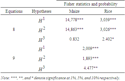
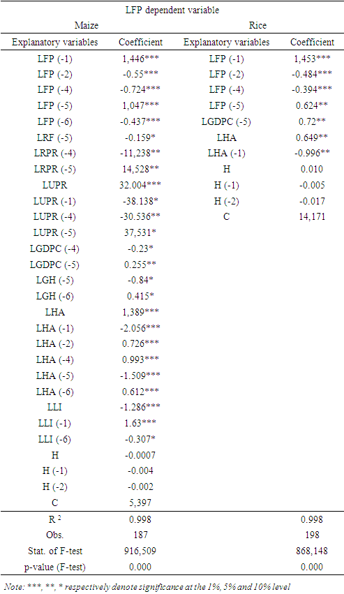
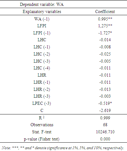
The results indicate that all the factors included in the model together significantly account for production at a rate of 99%. Regarding individual significance, production is influenced by previous quarters' production levels, rainfall, rural and urban populations, level of development (GDP per capita), sown area, land equipped with irrigation infrastructure, and gas emissions. The following Table 7 presents the contributions of the significant variables and the volatility of the model from Equation 8.

Table 7. Estimation results of the model of Equation 8 for Burundi

The results from Table 7 show that price volatility for rice and maize during the study period does not significantly affect their production in the selected countries, although the overall effect is negative. This aligns with findings from [44] and [45] in developing countries, suggesting that extreme price fluctuations surpass the threshold that would normally incentivize increased production. Climate variables—precipitation, temperature, and greenhouse gas (GHG) emissions—have no significant impact on rice production but do affect maize. Specifically, GHG emissions have delayed and contradictory effects: a 1% increase in CO₂ equivalent leads to a 0.84% decrease in maize production after 18 months but a 0.41% increase after 20 months. This suggests CO₂ becomes beneficial only after six quarters.

Foreign trade shows no significant influence on production in this context. However, previous harvests have a strong positive effect: a 1% increase in production leads to a 1.44% increase in maize and 1.45% in rice in the next quarter. Unexpectedly, rural population growth initially reduces maize production (−11%) but later boosts it (+14%), likely due to a shift from dependency to activity. Urban population growth, in contrast, directly increases maize production by 32%, as cities offer markets and labour support.

GDP per capita growth positively affects rice (a 1% increase leads to 0.71% more production after 18 months) but has a mixed impact on maize. This may be because rice is a cash crop, while maize remains mostly subsistence. Irrigation infrastructure is dedicated mainly to rice, explaining why it does not significantly benefit maize. Yet, this specialization may push farmers to expand maize cultivation into new dryland areas. Lastly, land area expansion significantly increases production: 1% more land boosts rice output by 0.64% and maize by 1.38%.

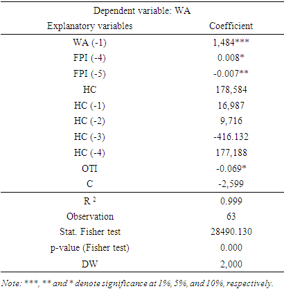
4.3.2. Food Utilization in Burundi

The factors considered in the model influence the prevalence of anaemia in women of childbearing age at 99%. The model is globally significant at 1%. The Ramsey specification, Breusch-Godfrey autocorrelation, and Breusch-Pagan-Godfrey heteroscedasticity tests confirm the robustness of these results. The following Table 8 indicates the relevant results of the study of equation 9.

Table 8. Estimation results of the model of Equation 9 for Burundi

The results of Table 8 make it possible to adjust the individual significance of the coefficients associated with the price volatility variables. Indeed, contrary to what was hoped, the prevalence of anaemia in women of childbearing age is positively balanced by the food production index. The growth of the food production index by 1% allows an increase in the prevalence of anaemia among women of childbearing age by 1.27%. This result shows that the situation of food insecurity can appear when production is abundant, which coincides with the analyses of Sen[46] on food accessibility. Even in the event of abundance, there are poor households (rural) whose purchasing power remains a limiting factor and still others who do not have access to a balanced diet because of multiple reasons such as ignorance, for example. All in all, this effect is somewhat attenuated by the production of the first delay (past quarter), which negatively influences anaemia in women of childbearing age by the effect of stocks. However, the price expected at production by farmers 3 quarters ago contributes to the reduction in the prevalence of anaemia among women of childbearing age. This is all the more understandable because the price of this same period contributes to the increase in production. In addition, these results let us see that in this study area, the prevalence of anaemia among women of childbearing age decreases every three times less than 0.006% during the period considered, and this decrease is significant.

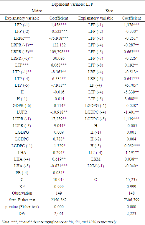
4.3.3. Food Availability in Kenya

In this study area, the determinants of the production of the two crops are, among others, previous production, precipitation, temperature, the number of fertilizers applied per hectare, the number of GHGs emitted, economic growth, the area sown, population growth, the area of land equipped with irrigation infrastructure, and GDP per capita. The variables taken together explain the variability of the production at 99%, and the joint significance is 1%, as shown by the Fisher test. The autocorrelation and heteroscedasticity test testify to the robustness of these model results. The following Table 9 illustrates the significant variables.

Table 9. Estimation results of the model of equation 8 for Kenya

The results in Table 9 indicate that current price volatility has a positive but statistically insignificant effect on rice and maize production. This is because production decisions are based on past experiences, with price signals observed before the cropping season. For rice, past volatility—especially from the first and third quarters—negatively affects production, as producers tend to redirect investments toward less risky crops, leading to lower yields. This supports the findings of [47] on rice and wheat in G7 countries. However, volatility in the second quarter positively influences rice production, aligning with [45], who observed that high volatility can sometimes drive economic growth in Sub-Saharan Africa.

Precipitation has divergent effects. For maize, current season rainfall significantly increases production (1 mm above average = + 0.15%) due to maize's rainfed nature. However, excess rainfall in the following quarter negatively impacts production (–0.29%), though this is often offset by current rainfall. For rice, excess rainfall reduces yield, particularly during sensitive growth stages, but delayed rainfall positively influences production by improving field conditions.

A temperature rise negatively affects both crops. A 1°C increase above average decreases maize and rice production by 1.556% and 8.48%, respectively, due to heat stress, which is particularly critical for rice during flowering.

Greenhouse gas (GHG) emissions have mixed effects. For maize, emissions directly boost production, contradicting [48]. For rice, GHGs show a delayed and contradictory impact: negative after 18 months but positive after 20 months. Overall, increased emissions harm long-term crop production under current environmental conditions.

Foreign trade has no significant effect on production. Instead, land area and fertilizer use are key drivers. A 1% increase in cultivated area boosts maize production by 1.31% and rice by 0.95%. Fertilizer residue also enhances future yields—1 ton/hectare increases production in the following quarter by 0.20% (maize) and 0.24% (rice).

Finally, rice production is strongly influenced by economic factors. A 1% increase in GDP per capita results in a 2.15% increase in rice production in the next quarter. Similarly, overall GDP growth in the current quarter supports rice production by enabling access to inputs. However, this same growth negatively affects rice output in the following quarter (–0.032%), possibly due to delayed policy or market adjustments.

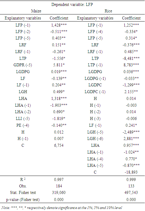
4.3.4. Food Utilization in Kenya

The prevalence of anaemia among women of reproductive age in Kenya is influenced mainly by the rate of anaemic women in the previous period, the consumer price index, the food production index, GDP per capita, the price volatility of rice and maize, the trade openness index, and population growth. These factors explain the prevalence of anaemia in women of childbearing age at 99%, and these contributions are significant at the 1% level. The following table shows the contributions of these significant variables, and the regression results are appended.

Table 10. Estimation results of the model of equation 9 for Kenya

The results in Table 10 show us that the price volatility of the two products has a significant influence on the rate of anaemia in women of childbearing age but to a different degree. Maize price volatility (HC) has a stronger influence on anaemia in women of reproductive age compared to that caused by rice. The uncertain increase occurring during a quarter of 1% in the price of 1 kg of maize causes an increase of 218% (weakly significant) among women of childbearing age, while it is 8% for rice (HR). The time required for the volatility observed in the market to contribute to the reduction in the rate of anaemia in women of childbearing age is approximately one year for both products. This is because there must be a time to produce, to make products available on the market, and to wait for the effect of the food consumed in the human body. After the 3^rd and 4^th quarters, the volatility of the price of maize contributes to the significant decrease in the rate of anaemia among women of childbearing age (556.14% and 395.36% respectively), while that of rice does not only contributes to a decrease of 17.3% after the 4^th quarter. This contribution of maize price volatility to the anaemia rate is not surprising because it has a positive influence on production. In other words, maize is the main commodity in this study area compared to rice.

During the period considered in the study, the results show that the prevalence of anaemia in women of childbearing age decreases gradually and significantly over time (0.04% each quarter). The fact that the crop production index negatively affects the rate of anaemia in women of childbearing age shows that the situation of food insecurity can coexist with the abundance of food products in a given area. These results corroborate those of [44] and reinforce the predictions of Sen [46]. Therefore, a situation of food insecurity is not only the result of insufficient national food production; it is also a problem of insufficient means of access to a balanced diet. Nevertheless, the abundance of production in one quarter can negatively influence the anaemia rate in women of childbearing age during the following quarter because the realization of stocks allows the increase in food availability on the market. The day after new harvests and leaving the nutritional state to another is a process that does not happen overnight.

With all hope, the level of development (GDP/capita) contributes to the reduction of anaemia in women of childbearing age. This result confirms those found by Kamgnia [28] and Fidoline associated with his collaborators [44], saying that per capita GDP decreases the rate of undernourishment. Conversely, population growth is a factor that positively influences the rate of anaemia among women of childbearing age since in developing countries, a certain number of households with many dependent children, in a situation of price instability, can reduce the number of meals per day or, to feel satiated, sacrifice quality for quantity; change eating habits by adopting cheaper and therefore less nutritious food. On the other hand, after a certain time, some children become adults and are ready to go about their activities, thus contributing to the reduction of undernourishment in the household. Another possible scenario is that of child labour in households to contribute to the survival of one's family. The trade openness index tends to increase the number of anaemic women. This is because this country exports most of its production to its northern neighbours, who are a potential food market. Moreover, this fact is advantageous for the following quarter since it acts as a factor in reducing the rate of anaemic women of childbearing age by encouraging producers to produce more.

4.3.5. Food Availability in Tanzania

In this study area, the analysis focused only on maize production due to a lack of data on rice prices. Maize production is then explained at 99% by all the factors of the model taken together. Autocorrelation and heteroscedasticity tests confirm the authenticity of these results. Individually, production is significantly influenced by past production, the quantity of fertilizers, economic growth, sown area, rural population, and the expected farm gate price.

Table 11. Estimation results of the model of equation 8 for Tanzania

As the results of Table 11 indicate, price volatility does not influence production. Indeed, the expected price elasticity of the second prior period of maize availability is 0.34. This shows that throughout the analysis, the instability of domestic maize prices positively affects the level of maize availability within the country. In other words, a variation of 1% in the expected price of maize on the domestic market leads to an increase of 0.34% in the level of maize availability. This result is consolatory for food security because producers are satisfied with the price received for their production, which encourages them to produce more.

Production is still positively balanced by economic growth. At the macroeconomic level, this result suggests that the more the country provides the necessary means to boost agricultural production, such as increasing the budget for the agricultural sector. Again, as expected, the area harvested contributes to the increase in the production of this crop. If the cultivated area varies by 1%, the production, in turn, varies by 0.54%. Conversely, the quantity of fertilizers does not intervene as expected. The negative sign of fertilizers in maize production can reveal two possibilities to us: the first is the most probable is the misuse of this input as stated by Mekuria [49] while the second possibility is the nature of the soils which are not compatible with the fertilizers used. In addition, as hoped, GHGs hinder production. The increase in GHGs of 1 T of CO₂ equivalent causes a decrease in production of 0.063%. As for the contribution of the rural population, it is doubtful and requires a rather specific interpretation. Only the second and the third periods contribute significantly but in a divergent manner to the variation in production. The variation of the rural population of 1% will cause an increase in production of 167% (significant at the 10% threshold) after 6 months, while after 9 months, it will cause a decrease of 167.343% (significant at 1% level). From the above, it is then obvious that the weight of the negative contribution is greater than the weight of the positive contribution. In short, the increase in rural population is not good news for food security because not only is there a higher dependency rate, but also, the more the rural population increases, the more arable land shrinks and, consequently, the more production. Due to the combination of all these factors, production increases over time, and producers strive to improve yields. This is noticeable through the inertia of production on itself. The results show that there is a 10% increase after each trimester.

4.3.6. Food Utilization in Tanzania

The prevalence of anaemia among women of childbearing age in this area is, among the criteria considered, significantly influenced by the food production index, the trade openness index, and the number of anaemic women.

Table 12. Estimation results of the model of equation 9 for Tanzania

Table 12 shows that price volatility does not have a significant influence on the prevalence of anaemia in women of childbearing age, but it is positive. If the prevalence of anaemia among women of childbearing age is decreasing in this region, it is thanks to factors such as the trade openness index. If the trade openness index increases by 1%, the prevalence of anaemia among women of childbearing age decreases by 0.069% every three months. This result tells us on the macroeconomic level that the country ensures that imports come to fill the internal deficit to lower the rate of malnourishment. This effect is increasingly reinforced by the action of the food production index, which, in addition to being an indicator of the importance of food in plant production, is also an indicator of food diversity. The positive effect of the production achieved begins to be noticed after five trimesters, while the effect of the 4^th quarter (weakly significant) causes an increase in the prevalence of anaemia in women of childbearing age.

4.3.7. Food Availability in Rwanda

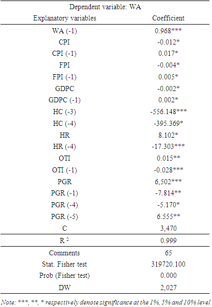
The local availability of the agricultural products considered in this study is, in this area, significantly influenced by the following factors: the entire population in general, population growth, GDP per capita, harvested area, areas equipped with irrigation, average annual temperature, and precipitation, foreign trade, expected producer price and price volatility.

Table 13. Estimation results of the model of equation 8 for Rwanda

In the study area, rice price volatility significantly affects local availability by negatively influencing production. A 1% increase in rice price leads to a 0.05% decrease in production after three quarters. In contrast, maize production is not significantly affected by price volatility but responds positively to expected prices at harvest; a 1% increase in expected price boosts production by 0.08% in the fourth quarter. This suggests that unpredictable price fluctuations undermine food security, whereas predictable prices motivate farmers to increase production.

Foreign trade plays a dual role: while imports improve short-term availability and stabilize prices, they may disincentivize local production by lowering market prices, thereby reducing farmer income. This dilemma is critical in developing countries where agriculture remains a primary livelihood source.

Population growth also constrains agricultural production. As confirmed by [49,50,51], and [52], a 1% rise in the rural population results in a 75% decline in maize production—mainly due to youth inactivity and land pressure. Urban population growth initially decreases maize output by 10%, but stimulates a 17% increase in the next harvest as producers adjust to rising demand.

Climatic conditions are crucial. According to Lobell & Gourdji [53], temperature and precipitation significantly affect crop yields. A 1°C rise increases maize yield by 6% initially but causes an 8% decline in the following quarter, likely due to water stress. Rainfall also shows time-dependent effects: excessive rainfall disrupts rice transplanting, leading to production losses, while well-timed rain in earlier periods improves soil moisture and benefits subsequent yields.

Development levels also influence agricultural output. A 1% increase in GDP per capita raises rice and maize production by 1.139% and 0.788%, respectively. However, as incomes grow, some farmers shift away from agriculture to other sectors like trade, potentially explaining negative effects. Finally, land expansion remains the most consistent driver of production growth, as extensification continues to be a key strategy in these rural settings.

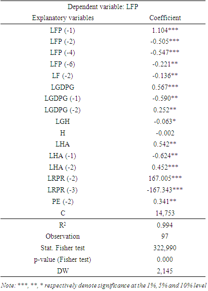
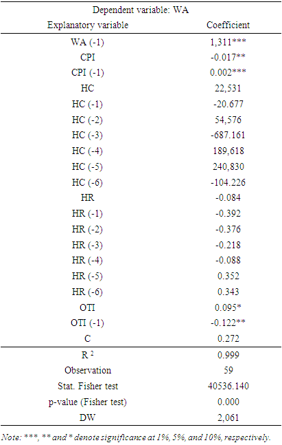
4.3.8. Food Utilization in Rwanda

The prevalence of anaemia among Rwandan women of childbearing age is strongly explained overall by the factors taken into consideration in the model at 99%. The diagnostic and specification tests of the model attest to the robustness of these results. In deducing individual significance, it is influenced by inflation and trade openness as the prevalence of anaemia in women of childbearing age.

Table 14. Estimation results of the model of equation 9 for Rwanda

Price volatility and producer prices do not have a significant influence. The elasticity of the trade openness index shows that following a 1% increase in the trade openness index, the prevalence of anaemia among Rwandan women of reproductive age will increase by 0.095% during this quarter. In the following quarter, it will decrease by 0.121%. This result tells us that, trade openness being a two-way index, foreign trade can influence positively on the one hand, or negatively on the other hand the prevalence of anaemia in women of childbearing age. If the country lets its production flow freely to the outside, it will create a food deficit inside and probably a high rate of undernourishment. Also, an increase in this index resulting from imports can firstly increase domestic availability and therefore reduce the rate of undernourishment among a certain segment of the population while decreasing the income of farmers, which will secondly cause a decline in local production and, in other words, an increase in undernourishment in poor households. In a rational production system, inflation is an incentive for production; hence, in this case, it discourages the prevalence of anaemia in women of childbearing age: an increase in inflation leads to a decrease of 0.017% in the prevalence of anaemia in women of reproductive age. Regarding the prevalence of anaemia in women of childbearing age who influence themselves, this result makes us think that there are women with anaemia who give birth to daughters who grow up with anaemia. This is a possible case in poor households.

5. Conclusion and Recommendations

Overall, the volatility of agricultural prices does not contribute significantly to food availability in the EAC, except in Rwanda, where it negatively and significantly influences the quantity of rice production. Overall, the negative influence of volatility dominates in the economy considered, however, it is the contrary in Kenya for maize production where it positively influences production. The non-significant influence is not to be taken as such, rather, its contribution is not perceived since farmers do not benefit from enough information from the agricultural market and its trends over time so that they can make an integration of the system's rational production. Farmers take into account only the expected price to boost production, while volatility is another factor contained in the price, which is a conditional variation of the market.

However, the influence of price volatility on food security can then be seen in the prevalence of anaemia among women of childbearing age with a positive influence. Price volatility especially discourages the accessibility of agricultural products, which is observed in this area where people suffer from undernourishment while there is a high index of food production.

Population growth and the factors responsible for climate change (rainfall, temperature, and greenhouse gas emissions) are imminent obstacles to food security in the region. Greenhouse gases negatively influence (after a year and a half) production.

The effects of foreign trade on food security vary according to a zone and according to a period. EAC countries, like other developing countries, are net importers. The food deficit is most often filled by imports, which often limit the performance of local producers and the integration of agricultural innovations to increase agricultural yields. As agriculture remains rainfed, the increase in production is the result of extensification in the region.

Based on the results of this study, the following recommendations can be made:

- Considering the effects of volatility that degrade the state of food security in the study area, countries should implement a price stabilization policy for necessities, especially by guaranteeing a remunerative price to producers and by making strategic stocks. It would also be all the more judicious to set up a platform disseminating information concerning the situation and the prediction of agricultural markets.

- Regarding imports and trade openness, which encourages the proliferation of undernourishment and poverty following the reduction of agricultural income, countries should control the flows and the nature of imported food products to put an end to the evolutionary figures of insecure people;

- Looking at the variables responsible for climate shocks that negatively influence production, countries should set up agricultural risk management funds to minimize risks and enable farmers to obtain credit from financial institutions;

- Concerning inflation, which increases the prevalence of anaemia among women of childbearing age, countries should control this factor to maintain purchasing power at an acceptable level and consequently reduce the rate of under- food in the area;

- Regarding the food production index, which encourages the prevalence of anaemia among women of childbearing age, the countries of the study area are requested to set up structures for sensitization on nutrition. (a healthy and balanced diet) to better control the proper use of food.

Finally, as a perspective, the researchers should continue the study on an area as vast as that considered in the present study, especially by using the raw data of short frequency. In addition, other researchers could investigate the determinants of agricultural price volatility in the study area.

6. Paper Limitations

The results of this study should be interpreted with several caveats in mind. First, due to data constraints, some EAC members—such as South Sudan and Uganda—were excluded, which reduced regional representativeness. Second, although it is methodologically logical, converting annual data to quarterly frequency could not effectively capture the effects of short-term volatility. Third, the lack of household-level data hinders our understanding of coping mechanisms and intra-national differences. Fourth, possibly due to farmers' limited access to market information, price volatility was often found to be statistically negligible. Fifth, factors related to trade and the environment do not account for more specific shocks, such as trade restrictions or severe weather. Finally, the findings' generalizability is limited by the impacts' variability among nations and crops, which necessitates additional regional assessments in subsequent studies.

Notes

1. This program is based on four pillars, which are: (i) extension of areas benefiting from sustainable land management and reliable water control; (ii) improvement of rural infrastructure and trade capacity for market access; (iii) increased food supply, to reduce hunger and improve response to food crises; and (iv) improved agricultural research, technology dissemination and adoption [54].

2. Here L represents the logarithm transformation.

3. In this equation, the variable of price volatility is subdivided into rice price volatility (HR) and maize price volatility (HC). It is the same for the variable PE where we have PEC for maize and PER for rice.