Omekara C. O. , Okereke O. E., Ukaegeu L. U.
Michael Okpara University of Agriculture, Umudike, Nigeria
Correspondence to: Omekara C. O. , Michael Okpara University of Agriculture, Umudike, Nigeria.
| Email: |  |
Copyright © 2016 Scientific & Academic Publishing. All Rights Reserved.
This work is licensed under the Creative Commons Attribution International License (CC BY).
http://creativecommons.org/licenses/by/4.0/

Abstract
In this paper, autoregressive fractionally integrated moving average (ARFIMA) model was proposed and was used for modeling and forecasting of liquidity ratio of commercial banks in Nigeria. Augmented Dickey Fuller (ADF) test was used for testing stationarity of the series. The long lasting autocorrelation function of the data showed the presence of long memory structure, and the Hurst exponent test was used to test for presence of long memory structure. The Geweke and Porter-Hudak (GPH) method of estimation was used to obtain the long memory parameter d of the ARFIMA model. Alternatively, a suitable ARIMA model was fitted for the liquidity ratio data. On the basis of minimum AIC values, the best model was identified for each of ARFIMA and ARIMA models respectively. The models were specified as ARFIMA(5,0.12,3) and ARIMA(1,1,1). To this end, forecast evaluation for the two models were carried out using root mean square error (RMSE). Having compared the forecasting result of the two models, we concluded that the ARFIMA model was a much better model in this regard.
Keywords:
ARFIMA model, ARIMA model, Long-memory, Autocorrelation function, Liquidity ratio
Cite this paper: Omekara C. O. , Okereke O. E., Ukaegeu L. U. , Forecasting Liquidity Ratio of Commercial Banks in Nigeria, Microeconomics and Macroeconomics, Vol. 4 No. 1, 2016, pp. 28-36. doi: 10.5923/j.m2economics.20160401.03.
1. Introduction
The financial stability of a bank can be tested in many ways. One of the quickest ways to see how well a bank is performing is to use liquidity ratios. A bank is considered to be liquid when it has sufficient cash and other liquid assets together with the ability to raise funds quickly from other sources, to enable it to meet its payment obligations and financial commitments in a timely manner. Liquidity ratios are the ratios that measure the ability of a bank to meet its short term debt obligations. These ratios measure the ability of a bank to pay off its short term liabilities when they fall due. Liquidity ratios basically allow banks a way to gauge their paying capacity on a short-term basis.For modeling time series in the presence of long memory, the Autoregressive fractionally integrated moving average (ARFIMA) model is used. ARFIMA models are time series models that generalize ARIMA models by allowing non-integer values of the differencing parameter. The ARFIMA(p,d,q) model is a class of long memory models [1]; and [2]. The main objective of the model is to explicitly account for persistence to incorporate the long term correlations in the data. These models are useful in modeling time series with long memory that is, in which deviations from the long-run mean decay more slowly than an exponential decay.Alternatively, Autoregressive integrated moving average (ARIMA) model which is a generalization of an autoregressive moving average (ARMA) model would be employed in this study. They are applied in some cases where data show evidence of nonstationarity, where an initial differencing step can be applied to remove the nonstationarity. The model is generally referred to as an ARIMA (p,d,q) model where p, d and q are non-negative integers that refer to the order of the autoregressive, integrated and moving average parts of the model respectively.In this study, we shall identify the order of ARIMA and ARFIMA models respectively, estimate the parameters of the two models, make relevant forecast based on the models, and compare the forecasting performance of the two models so as to know the better model in this regard.The rest of the paper is organized as follows. In section 2, we briefly present some theoretical framework on ARFIMA models. Materials and methods are discussed in section 3. In section 4, we analyze the underlying data and establish ARFIMA and ARIMA models on it. Finally the conclusions are presented in section 5.To our knowledge, ARFIMA models have not been used substantially to model liquidity ratios. This is therefore one of the contributions of this research.
2. Theoretical Framework
Financial data exhibit characteristics that are more consistent with long memory [4]. Long memory in time series are described as autocorrelation at long lags [3]. The ARFIMA model searches for a non-integer parameter, d, to differentiate the data to capture long memory. Regarding long memory, the useful entry points to the literature are the surveys by [3] and [4], who have described the development in the modeling of long memory on financial data, and of [5] who has reviewed long memory modeling in other areas. The existence of non-zero d is an indication of long memory and its departure from zero measures the strength of the long memory.One of the key points explained by [6] is the fact that most financial markets have a very long memory property. In other words, what happens today affects the future forever. This indicates that current data correlated with all past data to varying degrees. This long memory component of the market cannot be adequately explained by systems that work with short memory parameters. The general expression for ARFIMA processes  maybe defined by the equation:
 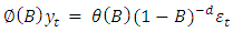 | (1.1) |
where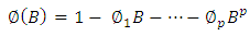 | (1.2) |
and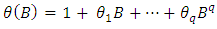 | (1.3) |
are the autoregressive and moving average operators respectively;B is the backward shift operator and  is the fractional differencing operator given by the binomial expression
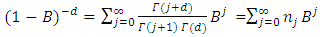 | (1.4) |
Short memory systems are characterized by using the last i values for making the forecast in univariate analysis. For example most statistical methods last i observation is given in order to predict the actual values at time i+1. Traditional models describing short-term memory, such as AR (p), MA (q), ARMA (p,q), and ARIMA (p,d,q), cannot precisely describe long-term memory. The general expression for ARIMA process  is defined by the equation.
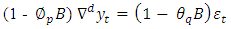 | (1.5) |
Where: 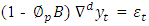 is the Autoregressive component
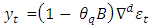 is the Moving Average component.
3. Materials and Methods
In this part of the study, the procedures for building ARFIMA(p,d,q) model and ARIMA model are discussed. Monthly data between January 2004 to December 2015 of the liquidity ratio data are used in the study. The presence of long memory process is tested on the data using the Hurst exponent since ARFIMA models are useful in modeling time series with long memory. When the integration parameter d in an ARIMA process is fractional and greater than zero, the process exhibits long memory [1]. Also in a class of stationary processes where the autocorrelations decay much more slowly over time than in the case of the ARMA processes or in the integrated processes long memory processes is also suspected.Conversely, ARIMA model which is a short term memory model will be used to model the liquidity ratio data and the forecasting performance of both ARFIMA and ARIMA shall be compared. To apply the ARFIMA and ARIMA models, the variables are first examined for stationarity. The Augmented Dickey Fuller (ADF) test is used for this purpose. This preliminary test is necessary in order to determine the order of non-stationarity of the data.The following methods will be used for the analysisAugmented Dickey Fuller (ADF) test:The ADF regression equation due to [7] and [8]is given by :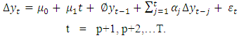 | (3.1) |
where  is the intercept,
  represents the trend incase it is present,
  is the coefficient of the lagged dependent variable,
  and p lags of
  with coefficients
  are added to account for serial correlation in the residuals. The null hypothesis
  is that the series has unit root while the alternative hypothesis
  is that the series is stationary. The ADF test statistic is given by
 where
where  is the standard error for
  and
and  denotes estimate. The null hypothesis of unit root is accepted if the test statistic is greater than the critical values.Testing for Long MemoryThere are various methods such as rescaled range analysis (R/S), modified rescaled range analysis (MRS), and De-trended fluctuation analysis (DFA), that are popularly employed for the recognition of a long memory. The Hurst exponent produced by rescaled range analysis is used in this study for testing long memory. The Hurst exponent was produced by a British hydrologist Harold Hurst in 1951 to test presence of long memory. The main idea behind the R/S analysis is that one looks at the scaling behavior of the rescaled cumulative deviations from the mean. The R/S analysis first estimates the range R for a given n:
 | (3.2) |
where,  is the range of accumulated deviation of
  over the period of n and
  is the overall mean of the time series. Let S(n) be the standard deviation of Y(t) over the period of n. This implies that;
 | (3.3) |
As n increases, the following holds: | (3.4) |
This implies that the estimate of the Hurst exponent H is the slope. Thus, H is a parameter that relates mean R/S values for subsamples of equal length of the series to the number of observations within each equal length subsample. H is always greater than 0. When  the long memory structure exists. If
  the process has infinite variance and is non-stationary. If 0 < H < 0.5, anti-persistence structure exists. If H = 0.5, the process is white noise.Estimation of long memory parameter For estimating the long memory parameter, GPH estimator proposed by Geweke and Porter-Hudak (1983) will be used in the present investigation. A brief description of the method is given below: This method is based on an approximated regression equation obtained from the logarithm of the spectral density function. The GPH estimation procedure is a two step procedure, which begins with the estimation of d. This method is based on Least square regression in the spectral domain, exploits the sample form of the pole of the spectral density at the origin:
  To illustrate this method, we can write the spectral density function of a stationary model yt , t = 1 , … T as
 | (3.5) |
Where  is the spectral density of
  assumed to be a finite and continuous function on the interval
  Taking the logarithm of the spectral density function
  the log spectral density can be expressed as
 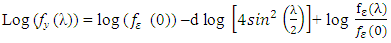 | (3.6) |
Let  be the periodogram evaluated at the Fourier frequencies
 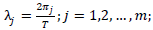 , T is the number of observations and m is the number of considered Fourier frequencies, that is the number of periodogram ordinates which will be used in the regression
  | (3.7) |
Where,  is a constant,
  is the exogenous variable and
 is a disturbance error. GPH estimate requires two major assumptions related to asymptotic behavior of the equation H1: for low frequencies, we suppose that log
  is negligibleH2: the random variables log [Iy (λj)]/ fy (λj)]; J = 1,2,…, m are asymptotically iid.Under the hypothesis H1 and H2 we can write the linear regression as
  Where
Where  Let
Let  the GPH estimator is the OLS estimate of the regression
  on the constant
  The estimate of d is given by the equation below:
 | (3.8) |
Where,  [3], [9] and [10] have analyzed the GPH estimate in detail. Under the assumption of normality for yt, it has been proved that the estimate is consistent and asymptotically normal.Information CriterionThe Akaike information criterion (AIC) is a measure of the relative goodness of fit of a statistical model. [11] suggests measuring the goodness of fit for some particular model by balancing the error of the fit against the number of parameters in the model. It provides the measure of information lost when a given model is used to describe reality. AIC values provide a means for model selection and cannot say anything about how well a model fits the data in an absolute sense. If the entire candidate models fit poorly, AIC will not give any warning of that.The AIC is defined as
  | (3.9) |
where k is the number of parameters in the statistical model, and L is the maximized value of the likelihood function for the estimated model. The AIC is applied in model selection in which the model with the least AIC is selected as the best candidate model.Root Mean Square Errors (RMSE):To construct the RMSE, we first need to determine the residuals. Residuals are the difference between the actual values and the predicted values, denoted by  where
where  is the observed value for the ith observation and
  is the predicted value. They can be positive or negative, depending on whether the predicted value under or over estimates the actual value. Squaring the residuals, averaging the squares, and taking the square root gives us the Root Mean Square Errors (RMSE). The RMSE will then be used as a measure to check the forecast accuracy of ARFIMA and ARIMA models respectively after which a more parsimonious model would be chosen. The Root Mean Square Error is given by:
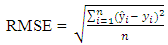 | (3.10) |
4. Results and Discussions
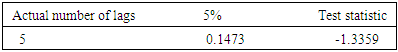
In this section, the monthly liquidity ratio series for the period January 2004 to December 2015 are analyzed using the ARIMA and ARFIMA models. The data are collected from Central Bank of Nigeria (CBN) statistical bulletin. Initial analysis of data: A time plot of the original series is shown in Fig 1. A visual inspection of the plot shows that the series is not stationary. In order to test for stationarity, Augmented Dickey Fuller unit root test [8] is conducted, and the result of ADF test is given in Table 1.Table 1. Result of the ADF test for stationarity
 |
| |
|
Structure of autocorrelationsFor a linear time series model, typically an autoregressive integrated moving average [ARIMA(p,d,q)] process, the patterns of autocorrelation and partial autocorrelation could indicate the plausible structure of the model. At the same time, this kind of information is also important for modeling non-linear dynamics. The long lasting autocorrelations of the data suggests that the processes are non-linear with time-varying variances. The basic property of a long memory process is that the dependence between the two distant observations is still visible. For the series on liquidity ratios of commercial banks in Nigeria, autocorrelations are estimated up to 100 lags, i.e j=1,…,100. The autocorrelation function of this series is plotted in figure 2.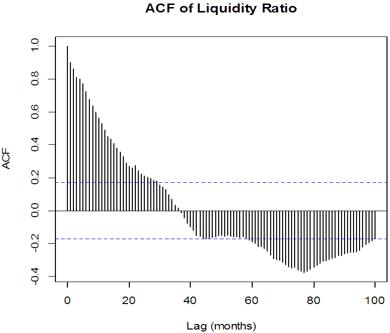 | Figure 2. Autocorrelation function of liquidity ratio of commercial banks in Nigeria |
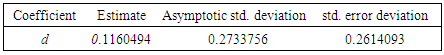
A perusal of Figure 2 indicates that autocorrelation function do not decay exponentially over time span, rather there is a very slow decay much slow than an exponential decay and it shows no clear periodic patterns. There is no evidence that the magnitude of autocorrelations became small as the time lag, j, became larger. No seasonal and other periodic cycles were observed. Testing for stationarityTo check stationarity in the series, the Augmented Dickey Fuller (ADF) test is mostly used as described in [7]. The first stage in model estimation is to test for the stationarity property of the data. The ADF test examines the null hypothesis that a time series Yt is stationary against the alternative that it is non-stationary.Table 1 contains the summary of results of Augmented Dickey Fuller test, Since the value of the computed ADF test statistic is smaller than the p-value at 5% level of significance, we conclude that the series is stationary at first difference.Testing for long memoryThe presence of long memory were tested using Hurst exponent (H) produced by the Rescaled range analysis. All steps of the calculation of H was done using programming techniques in R. The value of H was obtained to be 0.803984 indicating that the liquidity ratio data has long memory structure since  Estimation of the long memory parameterThe long memory parameter d is estimated using the [12] method. The estimated value of the parameter, its asymptotic deviation value and regression standard deviation values are reported in table 2 below
Table 2. Result of Estimating the d parameter
 |
| |
|
After estimating the long memory parameter d, the degree of autocorrelation in the fractionally differenced liquidity ratio series is examined using the autocorrelation and partial autocorrelation function as shown in figure 3.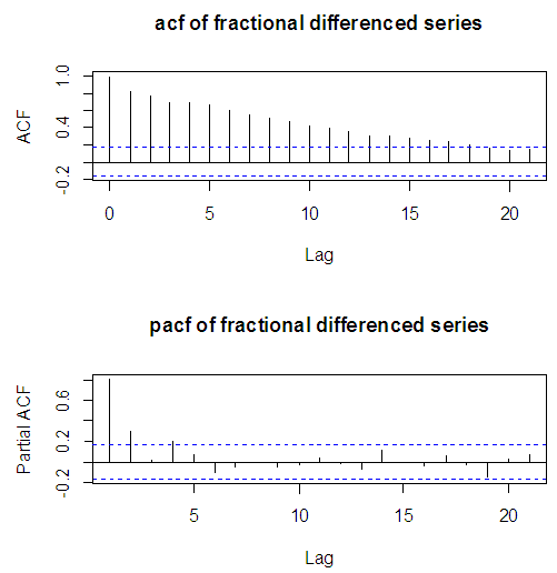 | Figure 3. ACF and PACF of fractionally differenced series |
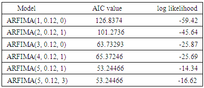
We move ahead to model the series as an ARFIMA process. First we start by identifying the ARFIMA model that best fits the series.ARFIMA model identificationThe optimal lag lengths for both the AR and MA are selected using the Akaike information criteria (AIC) and the log likelihood. Six candidate models are obtained. Out of these models a parsimonious model is obtained which has the lowest AIC and log likelihood function. The particular optimization routine of the log likelihood function shows that among the ARFIMA models that were tested, the optimal model for the fractionally difference series is ARFIMA(5, 0.12, 3) since this model exhibits the smallest values of AIC and log likelihood as reported in table 3 below.Table 3. Result of AIC and log likelihood tests
 |
| |
|
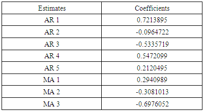
The result in table 3 shows that ARFIMA(5,0.12,3) model is the best candidate model with the least value of AIC and the log likelihood. After model identification, next is to estimate the parameters of the model.The result of the estimated parameters of ARFIMA(5,0.12,3) model are shown in table 4.Table 4. Result of the estimated ARFIMA(5,0.12,3) parameters
 |
| |
|
This calls for fitting of the model.The estimated parameters are fitted thus: | (4.1) |
 | (4.2) |
Having fitted a model to the fractionally differenced liquidity ratio time series, we check the model for adequacy.Diagnostic checking of ARFIMA modelThe model verification is concerned with checking the residuals of the model to see if they contained any systematic pattern which still could be removed to improve the chosen ARFIMA. This has been done through examining the autocorrelation and partial autocorrelation of the residuals. The residual ACF and PACF of the fitted ARFIMA(5,0.12,3) model of the fractionally differenced liquidity ratio time series are given in Fig.4 below.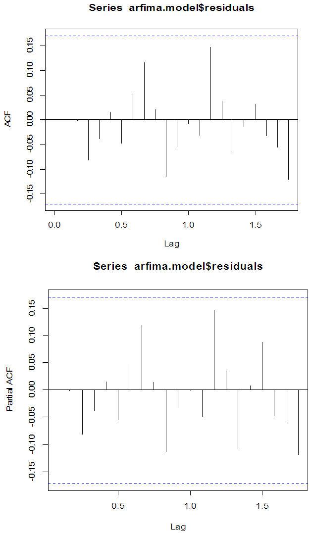 | Figure 4. Residuals ACF and PACF of ARFIMA(5,0.12,3) model |
The plots shows that there are no serial correlation observed in the residuals of the series, therefore the model is adequate and good.MODEL IDENTIFICATION USING ARIMA(p d q)An alternative way of modeling the liquidity ratio data is by fitting an ARIMA model. A visual inspection of the plot of the original series as conducted in figure 1 does not show any evidence of stationarity. Having discovered non-stationarity in the series, differencing at order 1 yielded a stationary series as shown in Fig 5 below.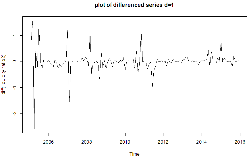 | Figure 5. Plot of first-order differenced series |
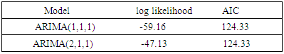
Since the series is stationary at order 1as shown in Figure 5, the optimal lag lengths for both the AR and MA are selected using the Akaike Information Criteria(AIC). Two candidate models are obtained using p=1,2; q=1. Out of these models a parsimonious model is obtained which has the lowest AIC and log-likelihood function. The value of the log likelihood and the AIC for two candidates ARIMA models are computed and reported in table 5.Table 5. Results of ARIMA model identification for liquidity ratio time series
 |
| |
|
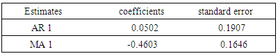
From the results obtained, the optimal model for the first order differenced series is ARIMA(1,1,1) since this model exhibits the smallest values of AIC and log-likelihood.ARIMA model estimationAfter the best model has been chosen, the parameters of the model are next estimated. The result of the parameter estimates of the optimal model are shown in Table 6.Table 6. Result of ARIMA model estimation for liquidity ratio time series
 |
| |
|
ARIMA(1,1,1) is fitted thus  | (4.3) |
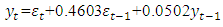 | (4.4) |
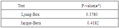
After fitting the model, we check for model adequacy.Diagnostic check of ARIMA(p,d,q) modelThe model is next tested for adequacy using two diagnostic tests namely; Ljung-Box test and Jarque-Bera test. The result of these test are given in Table 7.Table 7. Summary of diagnostic tests of ARIMA(1,1,1) model
 |
| |
|
The result of the test above, shows that the model is adequate at 5% as all the p-values are greater than 0.05. Also the residual ACF and PACF of the fitted ARIMA (1,1,1) model are given in figure 6 below.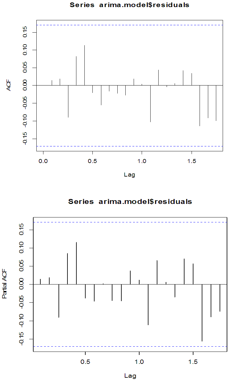 | Figure 6. Residual ACF and PACF of ARIMA(1,1,1) |
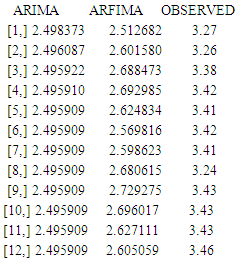
The plots shows that there are no serial correlation observed in the residuals of the series. Therefore ARIMA(1,1,1) is adequate.FORECAST EVALUATIONAfter checking the adequacy of ARIMA(1,1,1) and ARFIMA(5,0.12,3) respectively, we finally study their forecast values.A forecast result of ARIMA and ARFIMA models for the next 12 months were obtained. The result are shown in table 8.Table 8. Forecasting performance of ARFIMA and ARIMA models
 |
| |
|
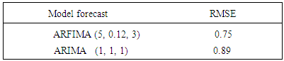
From the result above, the predicted values of ARFIMA(5,0.12,3) are closer to the observed values than the predicted values of ARIMA(1,1,1). In order to identify a more parsimonious model between the two types of models, we finally compare the forecast values of ARFIMA (5,0.12,3) and ARIMA (1,1,1) with the observed values. To evaluate their performance, Root mean squared error (RMSE) is used for this purpose.Table 9. Results of the benchmark evaluation for the two types of models
 |
| |
|
From the results above the RMSE value of ARFIMA (5,0.12,3) is smaller than the RMSE value of ARIMA (1,1,1), we therefore conclude that ARFIMA model is a much better model than the ARIMA model.
5. Conclusions
In this paper, we conducted a forecast of the liquidity ratio of commercial banks in Nigeria. The autocorrelation function of the liquidity ratio data showed persistence characteristic which is one of the features of a long memory process. This led to fitting a suitable ARFIMA(5, 0.12, 3) model.Similarly, the widely used ARIMA model was also employed in this study. A suitable ARIMA(1, 1, 1) model was identified and fitted. Even though both models fits the data well, forecasts obtained using the ARFIMA(5, 0.12, 3) model are closer to the actual values than forecasts obtained using ARIMA(1, 1, 1) model. It is also noteworthy that forecast evaluation using RMSE showed that the ARFIMA model is much better than the ARIMA model. We therefore conclude that liquidity ratio data is better modeled by ARFIMA model than ARIMA model.
References
| [1] | Granger C.W.J and Joyeux .R, 1980. An introduction to long memory time series models and fractional differencing. Journal of Time series Analysis, 15-29. |
| [2] | Hosking, J. “Modelling Persistence in Hydrological Time Series using Fractional Differencing”. Water Resources Research, 1984. |
| [3] | Robinson, P.M. (2003) Time Series with Long Memory. Oxford University Press, Oxford. |
| [4] | Baillie, R.T. 1996. Long memory processes and fractional integration in econometrics. Journal on Econometrics, 73: 5-59. |
| [5] | Beran, J. (1995) Statistics for Long Memory processes. Chapman and Hall Publishing Inc., New York. |
| [6] | Peters, E.E., 1991. Fractal market analysis- Wiley publishers, New York. |
| [7] | Dickey, D. and Fuller, W. (1979) Distribution of the estimators for autoregressive time series with a unit root. Journal of the American Statistical Association, 74: 427-431. |
| [8] | Said, S.E. and Dickey, D. (1984) Testing for unit roots in autoregressive moving average models with unknown order. Biometrika, 71: 599-607. |
| [9] | Hurvich, C.M., 2002. Multi-step forecasting of long memory series using fractional exponential models. International Journal of Forecasting. 18: 167-179. |
| [10] | Tanaka, K. (1999) The nonstationary fractional unit root. Econometric Theory, 15: 549-582. |
| [11] | Akaike, H. (1974). A new look at the statistical model identification. IEEE Transactions on Automatic control, 19(6): 716-723. |
| [12] | Geweke, J. and Porter-Hudak, S. (1983) The estimation and application of long-memory time series models. Journal of Time series Analysis, 4: 221-238. |

 Abstract
 Reference
 Full-Text PDF
 Full-text HTML