1. Introduction

It is commonplace to see several products sold as a combined product, say in a bundle. Firms in information, health care, telecommunication industries often offer products in bundles. Microsoft sells its word processor and spreadsheet in an office suite; many telecommunication companies sell the cables with their channels or services in bundles; Nintendo often offers the portable game console with a popular game in a single package. The problem of bundling attracts many economical researchers to discuss.

Many studies on bundling for multiproduct firms consider the products are complementary, such as cameras and lenses, computers and software. The one element cannot be used without another element, thus consumers must buy the products together (eg., Matutes and Regibeau,1988; Gans, J., and King, S., 2005). However, we consider the products are non-complementary and we earn different results from the previous work.

In Matutes and Regibeau (1988)’s model, they assumed there were two firms, A and B, selling two complementary system components, say, products 1 and 2. A consumer purchases at most one unit of each product. Therefore, when both firms engage in independent pricing, consumers have five options to select from, namely, AA, BB, BA, AB, and purchasing nothing. For example, AA means buying two components together from firm A, whereas AB means buying product 1 from firm A and product 2 from firm B. When both firms bundle, consumers have three purchasing options to select from, namely, AA, BB, and purchasing nothing. When only firm A bundles, because consumers must buy two components, the situation is the same as the one where both firms bundle. The researchers showed that independent pricing always dominated pure bundling.

In this study, we assume products are non-complementary-for example, like coffee and sugar. We can find a bundle of coffee and sugar in supermarket stores. However, coffee and sugar are also sold separately. A consumer may purchase only coffee because he prefers drinking coffee without sugar. A consumer may also buy the bundle for a lower price. Therefore, consumers are allowed to purchase only a single product in this situation. Based on the setup of Matutes and Regibeau (1988), with the new assumption that products are non-complementary, when both firms engage in independent pricing, there are nine purchasing options: AA, BB, A1, A2, B1, B2, AB, BA, and purchasing nothing. When only firm A bundles, consumers have AA, BB, B1, B2, and purchasing nothing to select from, which is not equal to the situation where both choose to bundle. In our study, we find that pure bundling may dominate independent pricing.

Moreover, we can analyze the monopoly market by extending the Matutes and Regibeau (1988)’s model. Based on the assumption that a monopoly holds non-complementary products, the incentive of bundling for a monopoly has been discussed and much of the work relies on the reservation price paradigm (e.g., Adams and Yellen 1976). However, different from the Hotelling model in Matutes and Regibeau (1988), Adams and Yellen (1976) built a two-dimensional model by assuming each axis represents consumers’ reservation price for either product. Consumers hold different level of reservation price for a product. In their result, they proved that whether bundling is more profitable depends on the distribution of customers in reservation price space. However, they concluded this by numerous experiments with continuous distribution of reservation prices and then they found that bundling dominates independent pricing in some occasions. In our two-dimensional Hotelling model, we can conclude the exact results by simple calculation, rather than numerous experiments.

By adding the possibility of consuming one product, Peitz (2008) analyzed the entry deterrence effect of pure bundling for a multiproduct monopoly in a two dimensional Hotelling model. This is not a symmetric market. In his model, consumers are allowed to buy a bundle from the incumbent in addition of another product from the rival if the entry has occurred. Based on this assumption, pure bundling is preferred by the incumbent if the entry has happened. This differs from the result of Whinston (1990) where bundling is never preferred if the entry has occurred. In Peitz (2008)’s model, the horizontal axis had vertical axis represent consumers’ willingness to pay from buying product 1 and 2, respectively. A consumer located further from a firm means that this consumer has higher willingness to pay of buying this firm’s product hence she is more willing to buy its product. However, in our model, a consumer located further from a firm means that she needs to pay more cost to buy the firm’ s product, therefore she is less willing to buy its product. Based on Peitz (2008)’s model, the market configuration does not change as consumers’ reservation changes. Nalebuff (2004) also considered the similar problem by assuming the incumbent chooses prices before the entrant in a two dimensional Hotelling model similar to our model. But he did not examine the change of the level of consumers’ reservation. However in our study, market configurations change as consumers’ reservation changes and we assume consumers buy at most of each product.

The remainder of this paper is arranged as follows. In section 2, the model and equilibrium in a monopoly market are introduced. In section 3 the model and equilibrium in a duopoly market are introduced. In section 4, we present a conclusion.

2. Monopoly Market

2.1. The Model

Suppose there are two products, product 1 and product 2. They are provided only by firm A. We assume the marginal cost of either product is zero. Firm A has two strategies to select from, that is, bundling and independent pricing. Consumers purchase at most one unit of each product. Therefore, consumers are able to select at most four consumption combinations if firm A does not bundle, namely AA, A1, A2 and purchasing nothing. AA means buying products 1 and 2 from firm A; A1, A2 mean purchasing only a single product 1 from firm A, a single product 2 from firm A respectively. Similarly, consumers are able to choose to buy AA or to buy nothing if firm A bundles. A consumer purchasing one product will have a reservation value or reservation price of C, which is the highest price she is willing to pay. Therefore, a consumer will have 2C if she purchases two products.

Consumers should be uniformly located in a Hotelling unit square with firm A located at (0, 0). In the unit square, product 1 is considered horizontally and thus as a consumer located further away from firm A horizontally, she holds less taste preference towards firm A’s product 1. Similarly, product 2 is considered vertically and as a consumer located further away from firm A vertically, she holds less taste preference towards firm A’s product 2. A consumer judges which combination she will buy by considering how much surplus she can get from purchasing each combination. Under an independent pricing scheme, a consumer located at (g₁, g₂) buying AA will get a surplus of 2C-λg₁-λg₂-p_1A-p_2A, where λ is the strength parameter of differentiation. p_1A, p_2A is the price of product 1 and product 2, respectively. Similarly, the consumer purchasing only a single product will get a surplus C-λg_m-p_mA, m=1, 2. When firm A bundles, the consumer buying the bundle will earn a surplus 2C-λ (g₁+g₂)-p_A, where p_A is the bundle price. We denote the profit under independent pricing as π_A^I, and the profit under bundling as π_A^B.

2.2. The Equilibrium Prices and Results

Our model is an extension of Matutes and Regibeau (1988). However, as explained above, consumers are able to purchase a single product in our model and this enable us to consider the problem in a monopoly market.

For simplicity of calculation, we set λ=1. We show the market configurations according to different levels of consumers’ reservation price (C) in Figure 1.

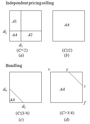Figure 1. Market configurations in a monopoly market

Under independent pricing, because the two products are assumed nonrelated, we can consider the market of product 1 and the market of product 2 separately. A consumer located at (g_1, g₂) will purchase A1 if C-λg₁-p_1A≥ 0, i.e., if she is located on the left side of the line g₁= C- p_1A. Similarly, the consumers located below the line g₂= C- p_2A will buy A2. As C increases, more and more consumers can afford to buy, and the duplicate area of AA becomes larger and larger. The market configurations may be (a) and (b) in Figure 1. Under bundling, a consumer located at (g_1, g₂) will purchase the bundle if 2C-λ (g₁+g₂)-p_A≥0, i.e., if she is located below the line g₂=2C-g₁-p_A. The market configurations under bundling may be (c) and (d). Let Q_1A and Q_2A, represent the demand of the product 1 and the demand of product 2 under independent pricing, respectively. Let Q_A represent the demand of the bundle. We list the equilibriums in Table1 and Table 2 and we show the calculations in the Appendix.

2.2.1. Independent Pricing

Table 1. The equilibriums under independent pricing

2.2.2. Bundling

Table 2. The equilibriums under bundling

2.2.3. Independent Pricing vs. Bundling

To observe which strategy is preferred, we analyze three cases. Firstly, we compare the equilibriums in (a) and (c) when C≤3/4. Then we compare (a) and (d) when 3/4≤C<2. Finally we compare (b) and (d) when C≥2. After the comparison of the profits and prices in the equilibriums, we find that when C<0.86, independent pricing dominates bundling, otherwise bundling is preferred. In addition, we find that when C<2^1/2, p_A< p_1A+ p_2A,, otherwise p_A≥ p_1A+ p_2A.

This result shows that the multiproduct monopoly may have different strategy according to different level of C. When C is relatively small, the firm has a stronger incentive to cut price if it bundles. In (a), decreasing the price of product 1 only increases the demand of product 1. Comparatively, in (c), decreasing the price of product 1 means decreasing the price of the bundle, and it will increase the demand of both products, thus p_A< p_1A+ p_2A. However, this price cutting effect just works when C is small and there are many potential consumers in the market (the blanked area). Cutting the bundle price can attract potential consumers. Moreover, consumers have more varieties like A1, A2 such single product when the firm does not bundle. This enables the firm to attract many consumers that cannot afford two products, and this single product does not exist under bundling. Therefore, when C is small, π_A ^B<π_A ^I.

As C increases, more and more people can afford to buy the products. And due to the price cutting effect, the potential consumers are less in the market of bundling compared with it in the market of independent pricing. However, as the potential consumers become less and less, cutting the price of the bundle will not increase the demand so much. Compared to cutting price to increase the demand, it is more profitable to increase the bundle price because the level of C is high enough to keep most people can buy the bundle. Similar to the price cutting effect, at this time, the incentive to increase the price under bundling is stronger than it under independent pricing. Thus p_1A+ p_2A < p_A. Moreover, as C increases, more and more people can afford two products in the market of independent pricing, thus the advantage of product variety is weakened. Therefore, we have π_A ^I<π_A ^B.

The price cutting effect disappears when there is a relatively small part of potential consumers under bundling, and then the firm chooses a higher price (which is higher than the sum of the prices in the market of independent pricing). Moreover, the price increases as C increases. Therefore, there is always a part of potential consumers feel difficult to buy the bundle. The market under bundling can never be fully served. Comparatively, under independent pricing, the price is always kept at a same level which is C/2 for each product. As C increases, the price increases and the market is gradually served more and more until fully served.

3. Duopoly Market

3.1. The Model

Suppose there are two products, products 1 and 2, which can be used together or separately, such as coffee and sugar. There are two firms in the market, firms A and B, producing both products 1 and 2. Without loss of generality, all marginal costs are set to equal zero. A consumer purchases at most one unit of each product. Therefore, if both firms engage in independent pricing, nine system configurations are available for consumers to purchase, as follows: AA, BB, A1, A2, B1, B2, AB, and BA; otherwise, they purchase none. For example, AB means buying product 1 from firm A and product 2 from firm B and A1 stands for buying only product 1 from firm A. We examine the firm’ choice of pricing schemes by employing a two-stage game. In stage one, the firms decide whether to bundle. In stage two, the firms set their prices simultaneously.

We extend the basic model of Matutes and Regibeau (1988), allowing consumers to purchase only one product. Consumers are uniformly distributed on the unit square: firm A is located on the origin (0, 0), while firm B is located at the point of coordinates (1, 1). The horizontal axis stands for product 1, and the vertical axis stands for product 2. Generally, under an independent-pricing scheme, a consumer buying only one product has a surplus of C - λd_mj - p_mj, where m = 1, 2, and j = A, B. The term C is the reservation value common to all consumers to buy one product. Therefore, buying two products will result in 2C. The term d_mj is the distance between the consumer’s location and the firm j horizontally or vertically, which depends on the product m. The term p_mj is the price of firm j’s product m, and λ > 0 measures the degree of horizontal product differentiation. We assume λ = 1 in this study. A consumer buying two products together has a surplus of 2C - λ(d_1i + d_2j) - p_1i - p_2j, where i, j = A, B. Concerning different pricing schemes, if a consumer buys both products from firm i engaging in pure bundling, she will have a surplus of 2C - λ(d_1i + d_2i) - p_i, where p_i stands for the price of pure bundling of firm i.

3.2. The Equilibrium Prices and Results

The market configurations corresponding to different dimensions of C are presented in Figure 2. The three strategy combinations possible are BB, BN (NB), and NN. BB means that both firms engage in pure bundling. BN means only one firm engages in pure bundling, and we set the condition that firm A is the one that does so. NN is the combination that both firms do not bundle goods. Concerning the situation where only firm A bundles, we demonstrate an example for the calculation in the situation where C ≤ 1/2. The demand of AA on the horizontal and vertical axes are the same, and we denote demand as d_mA, m = 1, 2, and 2C - d_mA - p_A ≥ 0 (i.e., d_mA ≤ 2C - p_A). Then, the area of the triangle is (2C - p_A)²/2, and this is the demand for firm A. Therefore, profit is π_A = p_A (2C - p_A)²/2. Maximizing firm A’s profit with respect to p_A gives us maximized p_A* = 2C/3 and π_A* = 16C³/27. For other calculations, please refer to the Appendix.

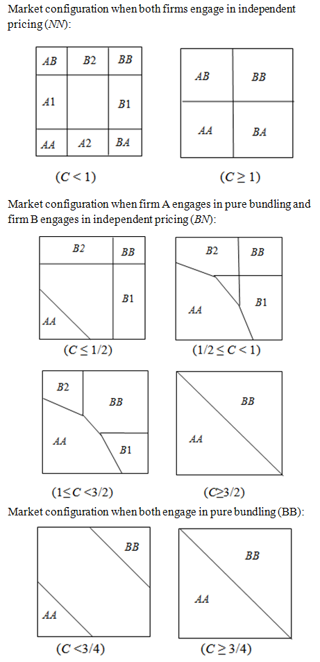Figure 2. Market configuration in a duopoly market

We define π^hl as the profit of a firm engaging in strategy h, while the rival engages in strategy l, with h, l∊{B, N}. The term p^hl is the price of one product but it is the bundle price when h stands for bundle (B). We obtain the equilibriums as follows:

As C is small, both firms choose independent pricing (NN):

When C < 1/2, because π^NN = π^NB > π^BB = π^BN, and

When 1/2 ≤ C < 3/4, because π^NN > π^NB > π^BB > π^BN.

We also have the results on the prices as follows:

2p^NN > p^BN = p^BB > p^NB = p^NN, when C < 1/2, and

2p^NN > p^BN > p^BB > p^NB = p^NN, when 1/2< C ≤ 3/4.

As C increases, there are two equilibriums where both firms choose independent pricing (NN) and both choose pure bundling (BB),

When 3/4 ≤ C < 1, because π^NN > π^BB > π^NB > π^BN,

When 1 ≤ C < 3/2¹, because π^NN > π^BB > π^BN > π^NB, and

When C ≥ 3/2, because π^NN > π^BB = π^NB = π^BN.

We have the results on the prices as follows:

2p^NB > 2p^NN > p^BN > p^BB > p^NB > p^NN when 3/4 ≤ C < 1,

2p^NN > 2p ^NB > p^BB > p^BN > p^NN > p^NB when 1 ≤ C < 3/2, and

p^BN = p^BB = p^NN when C ≥ 3/2.

Comparing our results with those of Matutes and Regibeau (1988), we find several differences. We find that the market configurations are more complicated in the presence of single-product consumption. In our study, we find the result that both firms bundle (i.e., BB) may appear in the equilibrium, while independent pricing always dominates as a selling strategy over pure bundling (NN) in Matutes and Regibeau (1988). When 3/4 < C < 1, the market for BB is an adjacent market. In an adjacent market, according to Matutes and Regibeau (1992, p.52, line36), “both firms set prices for their complete systems so as to leave consumers located at the common market boundary with exactly zero surplus.” The market boundary of AA and just touches that of BB. Firms A and B do not compete directly, but all the consumers in the market are covered. Comparatively, competition among pure, bundled, and single-product systems is fierce in the market for BN. Therefore, we see π^BB > π^BN and π^BB > π^NB temporarily.

4. Conclusions

We sought to analyze the incentive of bundling in both monopoly and duopoly market by considering the products are non-complementary. In a monopoly market, the results show that the incentive to bundle changes as conservation price changes. This reflects that the popularity of the products affects a monopoly’ s decision on bundling. This result has not been discussed in the previous work. In a duopoly market, we find that bundling may appear in the equilibrium. We did not discuss the welfare due to the complexity of calculation and this could be the future topic.

Appendix

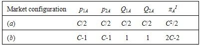
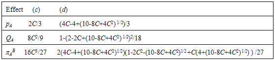
Monopoly market

1. The market configuration of (a)

Because the two products are independent, we can analyze them separately. In the market of product 1, we only consider horizontally. When the market configuration is as (a), the consumer (d1, 0) located in the boundary between to buy and not to buy A1 will earn a surplus of C- d₁-p_1A= 0 (i.e., d₁= C – p_1A). d₁ is also the demand of product 1. Then we get the profit from market 1 is (C- p_1A) p_1A. Maximizing this profit with respect to p_1A gives us maximized p_1A = C/2, Q_1A = C/2 and π_1A = C²/4. Then we can conclude the result in the market of product 2 by considering vertically, and we get the same result of maximized p_2A = C/2, Q_2A = C/2 and π_2A = C²/4. Therefore the total profit is π_A^I =π_1A+π_2A= C²/2. We can see that d₁ = d₂= Q_1A = Q_2A =C/2, when C=2, the market will be fully served to (b).

2. The market configuration of (b)

In (b), considering the market of product 1, firm A sets a price to ensure all consumers (equal to 1) to buy product 1 thus C-1-p_1A=0, and then we have p_1A= C-1, π_1A= C-1. Similarly, we have p_2A = C-1, π_2A= C-1. The total profit is π_A^I =π_1A+π_2A=2C-2

3. The market configuration of (c)

In (c), the consumer (d₃, 0) located in the boundary between to buy and not to buy AA in the horizontal line obtains a surplus of 2C –d3 – 0 – p_A = 0 (i.e., d3=2C - p_A). Similarly, we have d₄ = 2C - p_A in the vertical line. Then, the area of the triangle is (2C - p_A)²/2, and this is the demand Q_A for firm A. Therefore, the profit is π_A = p_A (2C - p_A) ²/2. Maximizing firm A’s profit with respect to p_A gives us maximized p_A = 2C/3, d3= d₄=4C/3, Q_A =8C²/9 and π_A^B = 16C³/27. We can see that d3= d₄=4C/3, when C=3/4, the market will change to (d).

4. The market configuration of (d)

In (d), for the consumer located at (y, 1), her surplus is 2C-dxy-1- p_A =0, then we get dxy=2C-1-p_A. Similarly we gave dzf=2C-1-p_A. Therefore the total demand Q_A is 1-(1-(2C-1-p_A)) ²/2, and the profit is p_A(1-(1-(2C-1-p_A)) ²/2). Thus we have the maximized p_A = (4C-4+(10-8C+4C²) ^1/2)/3, dxy=dzf=(2C+1-(10-8C+4C²)^1/2)/3,Q_A=1-(2-2C+(10-8C+4C²)^1/2)²/18 and π_A^B=2(4C-4+(10-8C+4C²) ^1/2)(1-2C²-(10-8C +4C²) ^1/2+C(4+(10-8C+4C²) ^1/2) ) /27. Because we find dxy = dzf = (2C+1-(10-8C+4C²) ^1/2)/3<1 always regardless of the level of C, thus as C increases, the market can never be fully served.

Duopoly market

The derivations of “both engage in pure bundling” can be found in Matutes and Regibeau (1988). Because there are a great number of market configurations and the ways of calculations are similar, we show two examples of how we derived the outcomes.

(1) When 1 ≤ C < 3/2, it is an adjacent market of NN in case 1, where the market boundary of AA and AB just touches, and the market boundary of AA and BA just touches. Since the market 1 is separated from market 2, therefore the market boundary of A1 and B1 just touches, A2 and B2 just touches. In an adjacent market, both firms set prices for their complete systems so as to leave consumers located at the common market boundary with exactly zero surplus. The markets of a certain product are symmetric, thus we have:

C-1/2-p_1A = 0, C-1/2 -p_1B = 0, C-1/2- p_2A = 0, C-1/2-p_2B = 0, so we have p_1A = p_1B = p_2A = p_2B = C-1/2. π_A = p_1A/2₊p_2A/2 = C-1/2, π_B = p_1B/2+ p_2B/2 = C-1/2.

(2) When 1/2 ≤ C < 1, we consider the market where only firm A engages in pure bundling in case 1. First, we can find the critical point where buying AA is indifferent from buying B2 for the consumer (0, g₂): 2C- p_A- g₂=C-p_2B-(1- g₂),, so g₂= (C+ p_2B +1- p_A)/2. Similarly we can find other critical points located on the axis. In addition, we can find the line where AA is indifferent from B2, where 2C- p_A- g₁- g₂ =C-(1- g₂) - p_2B, so g₁ = (1+C+ p_2B- p_A -2g₂). g₁, g₂ stand for the consumers located on the line in the unit square horizontally and vertically, respectively. We find the demand for each firm by using the critical points and indifference lines. The first order conditions are:

(A) (-9C²-3 p_1B ²-(1+ p_A)²-4 p_1B (3+ p_A)+2C(5+6 p_1B +3 p_A))/4

(B) (-9C²-3 p_2B ²-(1+ p_A)²-4 p_2B (3+ p_A)+2C(5+6 p_2B +3 p_A))/4

(C) (-2-10C²- p_1B ²-2 p_2B - p_2B ²-8 p_A -4 p_2B p_A -2 p_1B (1+ p_A)+2C(6+3 p_1B +3 p_2B +4 p_A))/4

The equations of (A) (B) and(C) can be solved by computer for several values of C.

Note

1. Strictly speaking, when C approaches 1.4, say C = 1.48, only NN becomes the equilibrium.