Pankaj Aswal1, Mangey Ram2, Manish Singh1
1Department of Management, Graphic Era University, Dehradun, 248002, India
2Department of Mathematics, Graphic Era University, Dehradun, 248002, India
Correspondence to: Mangey Ram, Department of Mathematics, Graphic Era University, Dehradun, 248002, India.
| Email: |  |
Copyright © 2012 Scientific & Academic Publishing. All Rights Reserved.
Abstract
Prices and quantities have been described as the most directly observable attributes of goods produced and exchanged in a market economy. The theory of supply and demand is an organizing principle for explaining how prices coordinate the amounts produced and consumed. In microeconomics, it applies to price and output determination for a market with perfect competition, which includes the condition of no buyers or sellers large enough to have a price-setting power. In this paper we analyze, the definition of non-linearization between the partial derivative (money, taxes, and quantity) is concluded to a set-point, which is optimized of all the three major partial derivatives governing the constraint of any economy by using Matlab programming.
Keywords:
Set-point, GDP Analysis, Optimization, Market Segmentation, Simulation Using Matlab, Supply and Demand Management
Cite this paper:
Pankaj Aswal, Mangey Ram, Manish Singh, "Effect of Supply and Demand in Controlling GDP Using Matlab Programming", Microeconomics and Macroeconomics, Vol. 1 No. 4, 2012, pp. 39-42. doi: 10.5923/j.m2economics.20120104.01.
1. Introduction
According to the demand supply model, the demand curve practically follows the non-linear relationship; this is apart from the case we took as an ideal condition. The international market is very much dynamic and does not follow the static standardization; hence it is not a linear curve.The supply and demand model describes how prices vary as a result of a balance between product availability and demand. The graph depicts an increase[6] (that is, right-shift) in demand from D1to D2 where (D12) along with the consequent increase in price and quantity required to reach a new equilibrium point[6] on the supply curve (S)[7].For a given market of a commodity, demand is the relation of the quantity that all buyers would be prepared to purchase at each unit price of the good. Demand theory[20] describes that,’ constrained utility maximization' (with income and wealth as the constraints on demand)[8], basically segmentation of the market.According to the law of demand price and quantity demanded in a given market are inversely related. That is, the higher the price of a product, the less of it people would be prepared to buy of it (other things unchanged). As the price of a commodity falls, consumers move toward it from relatively more expensive goods (the substitution effect)[14]. In addition, purchasing power from the price decline increases ability to buy (the income effect). Other factors can change demand; for example an increase in income will shift the demand curve for a normal good outward relative to the origin[6].It is the relation between the price of a good and the quantity available for sale at that price. It may be represented as a table or graph relating price and quantity supplied. Producers, for example business firms, are hypothesized to be profit-maximizes[5], meaning that they attempt to produce and supply the amount of goods that will bring them the highest profit. Supply is typically represented as a directly-proportional[16] relation between price and quantity supplied (other things unchanged). The higher price makes it profitable to increase production[8]. Just as on the demand side, the position of the supply can shift; say for a change in the price of a productive input or a technical improvement.Market equilibrium occurs where quantity supplied equals quantity demanded, the intersection of the supply and demand curves in the figure above. At a price below equilibrium, there is a shortage of quantity supplied compared to quantity demanded. This is posited to bid the price up[18]. At a price above equilibrium, there is a surplus of quantity supplied compared to quantity demanded. This pushes the price down. The model of supply and demand predicts that for given supply and demand curves, price and quantity will stabilize at the price that makes quantity supplied equal to quantity demanded. Similarly, demand-and-supply theory[2] predicts a new price-quantity combination of a shift in demand (as in the figure), or in supply.For a given quantity of a consumer good, the point on the demand curve indicates the value, or marginal utility, to consumers for that unit. The corresponding point on the supply curve measures marginal cost, the increase in total cost to the supplier for the corresponding unit of the good[13]. The price in equilibrium is determined by supply and demand. In a perfectly competitive market[2], supply and demand equate marginal cost and marginal utility at equilibrium.On the supply side of the market, some factors of production are described as (relatively) variable in the short run. Other inputs are relatively fixed[18]. In the long run, all inputs may be adjusted by management. These distinctions translate to differences in the elasticity (responsiveness) of the supply curve in the short and long runs and corresponding differences in the price-quantity change from a shift in the supply or demand side of the market.The consumers as attempting to reach most-preferred positions, subject to income and wealth constraints while producers attempt to maximize profits subject to their own constraints, including demand for goods produced, technology, and the price of inputs. For the consumer, that point comes where the marginal utility of a good, net of price, reaches zero, leaving no net gain from further consumption increases[14]. Analogously, the producer compares marginal revenue (identical in price for the perfect competitor) against the marginal cost of a good, with marginal profit[2] the difference. At the point where marginal profit reaches zero, further increases in production of the good stop. For movement to market equilibrium and for changes in equilibrium, price and quantity also change "at the margin": more-or-less of something, rather than necessarily all-or-nothing.Demand-and-supply analysis is used to explain the behavior of perfectly competitive markets, but as a standard of comparison it can be extended to any type of market. It can also be generalized to explain variables across the economy; for example, total output[estimated as real GDP (Gross Domestic Product)][9] and the general price level, as studied in macroeconomics[2].Studying the qualitative and quantitative effects of variables that change supply and demand, whether in the short or long run is a standard exercise in applied economics. Economic theory may also specify conditions such that supply and demand through the market is an efficient mechanism for allocating resources[1, 3, 10, 11, 12, 15, 19, 21].In this paper the authors suggested a comparative study on on controlling GDP in each financial year after 2006-07[Reserve Bank of India,http://www.rbi.org.in/scripts/PublicationsView.aspx?id=14525] in India and found that linear rising characteristics of each variable major contributing in GDP. This charaterstic curve is simulated by Matlab programming.
2. Qualitative Economics
It refers to the representation and analysis of information about the direction of change (+, - or 0) in some economic variable(s) as related to change of some other economic variable(s). For the non-zero case, what makes the change qualitative is that its direction but not its magnitude is specified.Typical exercises of qualitative economics include comparative-static changes studied in microeconomics or macroeconomics and comparative equilibrium-growth states in a macroeconomic growth model. A simple example illustrating qualitative change is from macroeconomics. Let: GDP = nominal gross domestic product, a measure of national income.M =money supply.T = total taxes.Monetary theory gives a positive relationship between GDP the dependent variable and M the independent variable. Equivalent ways to represent such a qualitative relationship between them are as a signed functional relationship and as a signed derivative[9]:+GDP= f (M) or df(M)/dM >0Where the '+' indexes a positive relationship of GDP to M, that is, as M increases, GDP increases, and vice versa.Another model of GDP hypothesizes that GDP has a negative relationship to T. This can be represented similarly to the above, with a theoretically appropriate sign change as indicated[20]: GDP =f(T) or df(T)/dT <0That is, as T increases, GDP decreases, and vice versa. A combined model uses both M and T as independent variables. The hypothesized relationships can be equivalently represented as signed functional relationships and signed partial derivatives (suitable for more than one independent variable):+
  GDP=f(M,T) or df(M,T)/dM>0 , df(M,T)/dT<0Qualitative hypotheses occur in the early history of formal economics but only as to formal economic models from the late 1930s with Hicks's model[4] of general equilibrium in a competitive economy. A classic exposition of qualitative economics is Samuelson, 1947. There Samuelson[4] identifies qualitative restrictions and the hypotheses of maximization and stability of equilibrium as the three fundamental sources of meaningful theorems-hypotheses about empirical data that could conceivably be refuted by empirical data.
3. The New Model as a Set-Point
The following model suggested that the new approach, in which there are three variables M, T, Q. Where Q is the quantity.+  GDP= f(M,T,Q) (i) ∂f(M,T,Q)/∂M>0(ii) ∂f(M,T,Q)/∂T<0(iii) ∂f(M,T,Q)/∂Q> or<0The model indicates a quantity that sold or purchased in following country which is independent variable with reference to GDP. Thus with the help of simulation plotting the quantity.
3.1. Money Supply
It shows the linear relationship[17] as the curve tends to linear characteristics. As it plotted against time, the money we spend on the production of goods is regularly increasing in magnitude, other terms of partial differential remain constant. This is shown up by the red line in Fig. 2. (Fig. 1).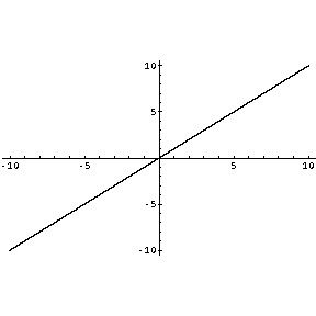 | Figure 1. Graph of money flow |
3.2. Taxes Imposed
It shows the parabolic output ,as taxes imposed tends to parabolic increasing characteristics[17], positive raising characteristics taxes imposed and negative decaying characteristics[6] shows that taxes decline as good does not exist. This is shown up by violet line in Fig. 2.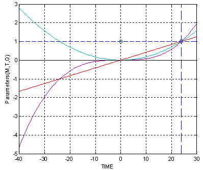 | Figure 2. Relationship among money, tax and quantity |
3.3. Quantity Supplied as Per Demand
Shows the exact parabolic raising characteristics if demand is positive and time is also positive the curve shows the rising positive pattern and increase in supply[6], If demand is positive and time is negative it is helpful in demand forecasting and helpful in setting production aim. This is shown up by the blue line in Fig. 4.
4. Algorithm for Fig. 2
1) Start 2) input variable M3) set values for M=(n up to 3 values)4) input variable T5) set values for T=(n up to 3 values)6) input variable Q=(n up to 3 values)7) take reference 08) produce set point9) apply positive set point10) regret negative set point11) execute the program12)endWhere (n) is the integer and finite number (i.e n=1,2,3…………………)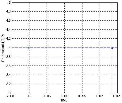 | Figure 3. Optimal parameter allocation (M,T,Q), set point-1 |
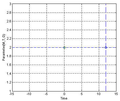 | Figure 4. Optimal parameter allocation (M,T,Q), set point-2 |
The set points we obtain with the help of Matlab programming software as shown below, the 2 positive set points. In Fig. 3 and Fig. 4, there are two different possible set-points after substituting the parameters M, T, Q.
5. Conclusions
This is advisable that to fix certain set-points in an outflow & inflow of goods as it controls the GDP. This analysis of Matlab programming is suitable for viable control a GDP and input many key important goods (as 16 products are major contributed in a control of GDP), as the variable via simulation process and a suitable part of cash inflow and outflow, to take the organizational goal setting the set point keep the track of optimal usage of different parameters and its deviation from the desired output.
References
| [1] | Anyadike-Danes, Michael and Godley, W. (1989) Real Wages and Employment: A Sceptical View of Some Recent Empirical Work, Machester School 62 (2):172-187. |
| [2] | Bouman, John (2011) Principles of Microeconomics - free fully comprehensive Principles of Microeconomics and Macroeconomics texts. Columbia, Maryland. |
| [3] | Brownlie, A. D. and Lloyd Prichard, M. F. (1963) Professor Fleeming Jenkin, 1833-1885 Pioneer in Engineering and Political Economy, Oxford Economic Papers, NS, 15(3), p. 211. |
| [4] | Cohen, A. J. (1983) The Laws of Returns Under Competitive Conditions': Progress in Microeconomics Since Sraffa (1926)? Eastern Economic Journal 9(3): 213-220. |
| [5] | Dutt, Amitava K. and Skott, Peter (2005) Keynesian Theory and the AD-AS Framework: A Reconsideration, Working Papers 2005-11, University of Massachusetts Amherst, Department of Economics. |
| [6] | Fleeming Jenkin, 1870 The Graphical Representation of the Laws of Supply and Demand, and their Application to Labour, in Alexander Grant, ed., Recess Studies, Edinburgh. ch. VI, pp. 151-85. Edinburgh. |
| [7] | Garegnani, P. (1970) Heterogeneous Capital, the Production Function and the Theory of Distribution, Review of Economic Studies 37 (3): 407-436. |
| [8] | Hagendorf, Klaus (2009) Labour Values and the Theory of the Firm. Part I: The Competitive Firm. Paris: EURODOS. |
| [9] | Hirshleifer, Jack, Glazer (2005) Amihai, and Hirshleifer, David, Price theory and applications: Decisions, markets, and information. Cambridge University Press, 7th Edition. |
| [10] | Hosseini, Hamid S. (2003) Contributions of Medieval Muslim Scholars to the History of Economics and their Impact: A Refutation of the Schumpeterian Great Gap. In Biddle, Jeff E., Davis, Jon B., Samuels, Warren J. A Companion to the History of Economic Thought. Malden, MA: Blackwell. pp. 28–45[28 & 38]. doi:10.1002/9780470999059.ch3. ISBN 0631225730. |
| [11] | Humphrey, T. M. (1992) Marshallian Cross Diagrams and Their Uses before Alfred Marshall, Economic Review, Mar/Apr, Federal Reserve Bank of Richmond, pp. 3-23. |
| [12] | Kirman, A. (1989) The Intrinsic Limits of Modern Economic Theory: The Emperor has No Clothes, The Economic Journal 99 (395): 126-139, Supplement: Conference Papers. |
| [13] | Lawrence, S. Ritter, William L. Silber, and Gregory F. Udell (2000). Principles of Money, Banking, and Financial Markets (10th ed.). Addison-Wesley, Menlo Park C. pp. 431–438, 465–476. ISBN 0-321-37557-2. |
| [14] | McGuigan, James R. Moyer, R. Charles and Frederick H. Harris (2001). Managerial Economics: Applications, Strategy and Tactics. South-Western Educational Publishing, 9th Edition. |
| [15] | Moore, Basij J. Horizontalists and Verticalists: The Macroeconomics of Credit Money, Cambridge University Press, 1988. |
| [16] | Opocher, A. and Steedman, I. (2009) Input Price-Input Quantity Relations and the Numeraire, Cambridge Journal of Economics 3:937-948. |
| [17] | Rogers, Colin (1989) Money, Interest and Capital: A Study in the Foundations of Monetary Theory, Cambridge University Press. |
| [18] | Rosen, Harvey (2005) Public Finance, p. 545. McGraw-Hill/Irwin, New York. ISBN 0-07-287648-4 |
| [19] | Samuelson, P. A. (2000) Reply in Critical Essays on Piero Sraffa's Legacy in Economics (edited by H. D. Kurz) Cambridge University Press. |
| [20] | Vienneau, R. L. (2005) On Labour Demand and Equilibria of the Firm, Manchester School 73(5): 612-619. |
| [21] | White, G. (2001) The Poverty of Conventional Economic Wisdom and the Search for Alternative Economic and Social Policies, The Drawing Board: An Australian Review of Public Affairs 2 (2): 67-87. |
 Abstract
 Reference
 Full-Text PDF
 Full-Text HTML