Suhada O. Tayyeh, Saffa J. Abdul-Hussien
Technical College of Management, Iraq
Correspondence to: Suhada O. Tayyeh, Technical College of Management, Iraq.
| Email: |  |
Copyright © 2018 The Author(s). Published by Scientific & Academic Publishing.
This work is licensed under the Creative Commons Attribution International License (CC BY).
http://creativecommons.org/licenses/by/4.0/

Abstract
In this paper, aggregate planning strategies are discussed and a special structure of transportation models are investigated for the aggregate planning purpose of Baghdad Company for soft drinks. For the purpose of achieving the aims of this study, we will develop an optimal total production plan by determining the quantities of production necessary to meet the variable demand for a period of time in the medium term and at the lowest cost using the transportation model and then comparing the company's plan with the proposed plan by adopting specific criteria for determining the best. The study reached a set of conclusions, the most important of which is the development of an optimal production plan for the family of the product under study for the year 2018, and recommended the need to work according to the optimal plan proposed, which is better than the company's plan, since the total cost of production of the company and the unsold production cost of the company, Is greater than the corresponding costs reached by the optimal solution of the transport model.
Keywords:
Aggregate planning, Transportation model, Seasonal ARIMA, the bottom-up approach
Cite this paper: Suhada O. Tayyeh, Saffa J. Abdul-Hussien, Using Transportation Model for Aggregate Planning: A Case Study in Soft Drinks Industry, Journal of Logistics Management, Vol. 7 No. 1, 2018, pp. 11-46. doi: 10.5923/j.logistics.20180701.02.
1. Introduction
Aggregate production planning is concerned with determining the quantity and timing of production in the intermediate future to meet forecasted demand, it usually covers a time period ranging from 3 to 18 months. The main objective of aggregate planning is to minimize the total cost over the planning horizon. The plan must take into account the various ways a firm can cope with demand fluctuations as well as the cost associated with them. Typically a firm can cope with demand fluctuations by, changing the size of the work force by hiring and firing (thus allowing changes in the production rate), varying the production rate by introducing overtime and (or) outside subcontracting, accumulating seasonal inventories and planning backorders.These ways of absorbing demand fluctuations can be combined to create a large number of alternative production planning options. Costs relevant to aggregate production planning are basic production costs (material costs, direct labor costs, and overhead costs), costs associated with changes in the production rate and Inventory related costs. There are two extreme aggregate production plans, the just-in-time production plan and the production-smoothing plan.Sultana etal. in 2014 discussed aggregate planning strategies and then investigated a special structure of transportation model for the aggregate planning purpose of “Bangladesh Cable Shilpa Ltd, Khulna”. For this transportation problem, all the unit costs, supplies, demands & other values are taken from a case study. They determined forecasting demand values by using Single Exponential Smoothing Forecasting technique. TORA software is used to find the optimum cost by using transportation method. Chada in 2015 designed and developed a computer program to facilitate exploration of aggregate planning methods to obtain desirable cost attributes. The first phase is to design and develop a spread sheet with different cases such that each case will use a constant strategy throughout the period for that particular case and also sensitivity analysis is performed on the input variables with the help of macros in the spreadsheet. The second phase is developed in such a way that there is flexibility to select different strategies for each period. Rosemary etal. in 2016 examined transportation model of quantitative techniques for management. she argued that, managers must be aware of the quantity of available supplies, the quantities demanded and location to find the cost of transporting one unit of commodity from place to another. Conclusions were drawn and recommendation made that the optimal solution to a transportation problems must consist of integer values for the decision variables as long as all supply and demand values are integers. Jamalnia in 2017 proposed a novel decision model to aggregate production planning decision making problem based on mixed chase and level strategy under uncertainty where the market demand acts as the main source of uncertainty. Jamalnia appraised also the performance of different aggregate production planning strategies in presence of uncertainty. Damghani etal. in 2017 proposed a multi-period multi-product multi-objective aggregate production planning (APP) model for an uncertain multi-echelon supply chain considering financial risk, customer satisfaction, and human resource training. They considered three conflictive objective functions and several sets of real constraints. Some parameters of the proposed model are assumed to be uncertain and handled through a two-stage stochastic programming (TSSP) approach. The proposed TSSP is solved using the goal attainment technique, the modified ε-constraint method, and STEM method. They applied the whole procedure in an automotive resin and oil supply chain as a real case study wherein the efficacy and applicability of the proposed approaches are illustrated in comparison with existing experimental production planning method.
2. Statistical Tools
2.1. Seasonal ARIMA Model
SARIMA models are the most general class of models for forecasting a time series, since there too many phenomena that are follow to.. Seasonal ARIMA models are expressed in factored form by the notation ARIMA(p,d,q)(P,D,Q)s, where p is the number of autoregressive terms, d is the number of nonseasonal differences needed for stationarity, q is the number of lagged forecast errors in the prediction equation, P is the order of the seasonal autoregressive part, D is the order of the seasonal differencing, Q is the order of the seasonal moving-average process and s is the length of the seasonal cycle. Given a dependent time series  mathematically the ARIMA seasonal model is written as,
 | (1) |
where, C is a constant, θ’s and Φ’s are weighting parameters for the different nonseasonal lagged terms, θ*’s and Φ*’s are weighting parameters for the different seasonal lagged terms, B is the back shift operator  and e represents a random error term.
2.2. Transportation Model
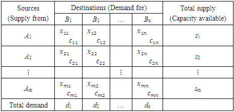
This model can be used for a wide variety of situations such as scheduling, production, investment, plant location, inventory control and many others.The transportation problem can be put in general form as shown in table (1)Table 1. Matrix of Transportation
 |
| |
|
Where,Ai – periods of production, i = 1,2, …,m (each period of production may contains production in regular time, production in overtime and production under subcontract), (the beginning inventory may be taken as first period of production)Bj – periods of demand, j = 1,2, …,nm – total number of containers producedn – total number of containers demandedcij –unit costs for the transport between i-th period of production and the j-th period of demand,i = 1,2, …,m, j = 1,2, …,nxij – number of containers supplied from i-th period of production to j-th period of demand,i = 1,2, …,m, j = 1,2, …,nsi – available number of produced containers at i-th period of production, i = 1,2, …,mdj – demand for containers at j-th period of demand, j = 1,2, …,n.It is worth mentioning that the costs concluded the regular production cost per unit, overtime cost per unit, subcontracting cost per unit, holding cost per unit period, Backorder cost per unit per period and inventory carrying cost. cij contains some of costs which are compatible with situation of xij . The mathematical model for the solution of the above transportation problem can be summarized as follows:Criteria function,  with constraints,
 | (2) |
 | (3) |
xij ≥ 0 ; i = 1,2, …,m, j = 1,2, …,n.To be conveniently correlated the equations (2) and (3) should fulfill the following condition: There are some assumptions in the transportation model, that are, total quantity of the item available at different sources is equal to the total requirement at different destinations, item can be transported conveniently from all sources to destinations, the unit transportation cost of the item of the item from all sources to destinations is certainly and precisely known, the transportation cost on a given route is directly proportional to the number of units shipped on that route and the objective is to minimize the total transportation cost.The first step to solve transportation problem is to find out the initial feasible solution. The Vogel approximation method (VAM) is an iterative procedure for computing that basic feasible solution. This method is preferred over the other methods, because the initial basic feasible solution obtained by this method is either optimal or very close to the optimal solution. The steps in VAM are as follows, 1. Identify the boxes having minimum and next to minimum transportation cost in each row and write the difference (penalty) along the side of the table against the corresponding row.2. Identify the boxes having minimum and next to minimum transportation cost in each column and write the difference (penalty) against the corresponding column3. Identify the maximum penalty. If it is along the side of the table, make maximum allotment to the box having minimum cost of transportation in that row. If it is below the table, make maximum allotment to the box having minimum cost of transportation in that column.4. If the penalties corresponding to two or more rows or columns are equal, you are at liberty to break the tie arbitrarily.5. Repeat the above steps until all restrictions are satisfied.After computing an initial basic feasible solution, one can used the modified distribution method (MODI) is for finding the optimal solution of a transportation problem. It is provides a minimum cost solution. The steps in MODI are as follows,1. Determine the values of dual variables, ui and vj, using ui + vj = cij 2. Compute the opportunity cost using cij – ( ui + vj ). 3. Check the sign of each opportunity cost. If the opportunity costs of all the unoccupied cells are either positive or zero, the given solution is the optimal solution. On the other hand, if one or more unoccupied cell has negative opportunity cost, the given solution is not an optimal solution and further savings in transportation cost are possible. 4. Select the unoccupied cell with the smallest negative opportunity cost as the cell to be included in the next solution. 6. Draw a closed path or loop for the unoccupied cell selected in the previous step. Please note that the right angle turn in this path is permitted only at occupied cells and at the original unoccupied cell. 7. Assign alternate plus and minus signs at the unoccupied cells on the corner points of the closed path with a plus sign at the cell being evaluated. 8. Determine the maximum number of units that should be shipped to this unoccupied cell. The smallest value with a negative position on the closed path indicates the number of units that can be shipped to the entering cell. Now, add this quantity to all the cells on the corner points of the closed path marked with plus signs, and subtract it from those cells marked with minus signs. In this way, an unoccupied cell becomes an occupied cell.
3. Case Study
To determine the optimal aggregate production plan, this will be according to the following subsections,
3.1. Prepare the Necessary Data
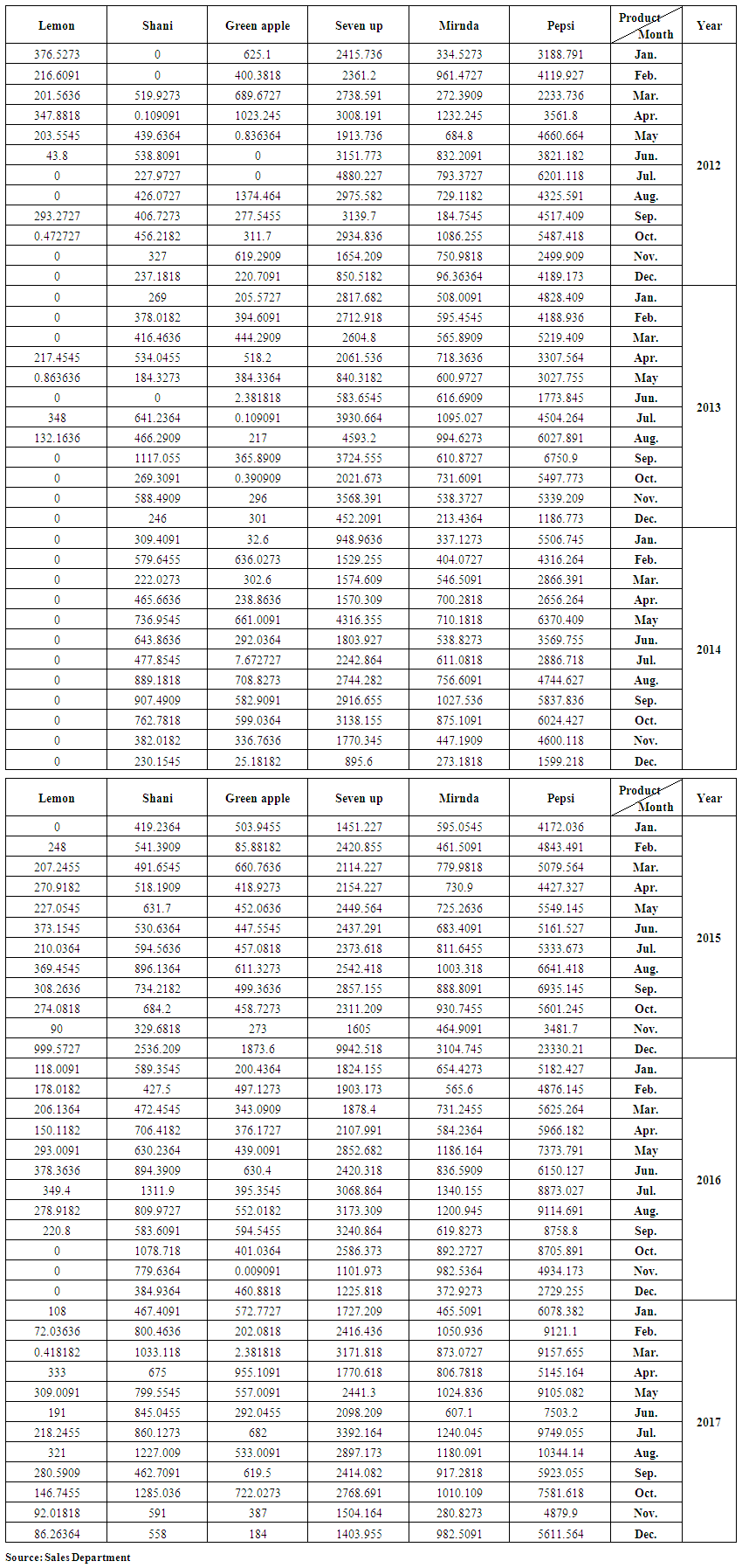
The data needed to achieve the aims of the study will be prepared as follows:1. For the purpose of conducting quantitative analysis appropriate to the objectives of the study, the monthly data for the demand and production of 250 ml (Pepsi, Miranda, Seven up, Green apple, peace, Shani, Lemon) for the period from the beginning of 2012 until the end of 2017 was obtained from Baghdad Company of soft drinks. This data is shown in tables (1-2) in annex respectively.2. Through the personal interview with the director of production operations and the administrator of the first line of production in Dijla plant, we learned that there are two of works shift, the first one starts from seven in the morning and ends at three in the afternoon (eight hours) and then extend for another two hours as an additional time until 5 pm. The second shift of the work begins from 7 pm to 3 am, followed by two additional working hours until 5 am. It is also worth mentioning that:a. The work shifts in Both of Fridays and Saturdays treated as additional shifts.b. Work is continuing for all days of the week except public holidays approved by the government and those granted to certain necessities. Table (3) In annex shows these holidays over the months from the beginning of 2012 until the end of 2017.3. Based on Table (3) In annex, the actual and additional working hours are in Table (4) In annex, were calculated for January 2012, for example, as follows:a. The number of regular working days (including additional working hours) is ((number of days of the month (31 days minus (8 days of Fridays and Saturdays plus an official holidays) 1 day of january (1 January) Remaining 22 days, 31 - 8 - 1 = 22.b. The additional working days (overtime) are (the number of Fridays and Saturdays, which is 8 days, minus a public holiday on Friday, (6th of January), which will be 8 - 1 = 7.c. The regular working hours are equal to the number of regular working days of 22 days multiplied by 16 hours (8 working hours for each shift), (22 x 16 = 352).d. The number of working hours for overtime is equal to the number of regular working days of 22 days multiplied by 4 hours (2 extra hours for each shift) plus 7 overtime days multiplied by 20 hours (10 overtime hours in each shift) (22 x 4) + (7 x 20) = 228. And so on for the rest of the months in the period under study from the beginning of 2012 until the end of 2017.4. According to table (4) In annex, we calculated the quantities of production within the regular and overtime hours of each of the products under study. These quantities are shown in tables from (5-10) In annex. for example, for December 2012, the calculations are as follows:a.The ratio of the number of regular work hours to the total number of working hours is, 352 / (580) = 0.606897.b. We multiply the above ratio by the number of containers produced of Pepsi in December 2012, the production quantity in regular time is, 0.606897 × 2199.327 = 1334.764. c. The ratio of the number of overtime hours to the total number of working hours is228 / (580) = 0.393103.d. We multiply the above ratio by the number of containers produced of Pepsi in December 2012, the production quantity in overtime is, 0.393103 × 2199.327 = 864.5631. And so on for the rest of the months and products for the period from 2012 to 2017.It is worth mentioning that the single container contains 110 boxes, each box contains 30 metal cans of 250 ml.
3.2. Demand and Production Forecasts
For the purpose of planning the aggregate production of the products of Baghdad Company for soft drinks and specifically for 250 ml metal cans for the period from March to December of 2018, firstly we will forecast the demand for those products as well as the quantities of production at the regular and overtimes in those months according to the following steps:1. Based on the demand data in Table (1) In annex and the quantities of production within the regular and overtimes in Tables (5-10) In annex, the Akaike criterion was used to determine the degree of appropriate model of data among several estimated models. In addition, the root of mean square error  is used to determine the advantage of a model among several models were estimated.a. The models mentioned in Table (11) In annex, are appropriate to represent the demand on containers for each product, and then the total demand for the sum of all products.b. The models mentioned in Table (12) In annex, are appropriate to represent quantities of production on containers for each product within the regular time, and then the total quantities of production for the sum of all products.c. The models mentioned in Table (13) In annex, are appropriate to represent quantities of production on containers for each product within the overtime, and then the total quantities of production for the sum of all products.It should be noted that the criterion for selecting the appropriate model is the least value of √MSE and the lowest value of the AIC criterion, for example SARIMA (1.0,0) x (2,0,0) 2, is a model which was chosen to represent demand. It was used to forecast future values for Pepsi, with value of √MSE equal to 2901.56 and value of Akiaki criterion equal to 1156.113, which are the lowest among all corresponding values of the models selected to represent the demand for Pepsi product.SARIMA (1,0,0) x (2.0.0) 2 model, which is represented the demand on the Pepsi, can be written according to the equation (1) as follows,
 | (4) |
The parameters values listed in Table (6) are substituted in the above equation to be, | (5) |
by writing, Equation (2) will be:
 | (6) |
Equation (6) above represents another form of the model in equation (4), and so it is for other models, whether for demand or production.2. Before using the models mentioned in Tables (11-13) In annex, for the purposes of forecasting, Box-Piers test were used to confirm the ability of chosen models to forecast. The Box-Piers test results that are shown in Tables (14-16) In annex, indicate that the ability of chosen models to forecast, where P value is the critical point between accept and reject the hypothesis that the model is able to forecast (there is no pattern for the residuals). The rule is accept the hypothesis where the chosen significant level is less than p. For example, p value for demand model on Pepsi product is 0.765096, Since this value is greater than all the common significant levels 0.01, 0.05 and 0.10, we accept the forecasts resulting from this model, and that the residuals are random.3. Using the models mentioned in Tables (11-13), the forecasts for the demand for the products under consideration, as well as the quantities of production at the regular and overtime for the months from March to December 2018, were obtained. Tables (17-19) In annex, shows the values of these forecasts.
3.3. Using the Transportation Model
After obtaining the previous data and information related with products under consideration beside the following information,1. Beginning inventory obtained from the company's stores for each product are in table (2),2. The production cost of single container in regular and overtime are 660,000 Iraqi dinars and 673000 respectively (from the final accounts of the company).3. The cost of storage of one container is 3000 Iraqi dinars per month (from the company's accounts).Table (2). Beginning inventory (containers) of the products under study on 1/3/2018
 |
| |
|
POM software was used to obtain the optimal value for the costs resulting from satisfying the demand of the products under consideration through the production of the company. The Vogel method was used to get initial basic feasible solution. The results are as follows,1. product (Pepsi): Table (20) In annex, represents the optimal solution for the transportation model. It is also includes the data and information that represent the analysis requirements to use the mentioned model. It was found that the lowest optimal cost value is 34975750000 Iraqi dinar.2. Product (Miranda): Table (21) In Annex, represents the optimal solution for the transportation model. It also includes the data and information that represent the analysis requirements to use the mentioned model. It was found that the lowest optimal cost value is 4850998000 Iraqi dinar.3. Product (Seven up): Table (22) In Annex, represents the optimal solution for the transportation model. It also includes the data and information that represent the analysis requirements to use the mentioned model. It was found that the lowest optimal cost value is 15484670000 Iraqi dinar.4. Product (green apple): Table (23) In Annex, represents the optimal solution for the transportation model. It also includes the data and information that represent the analysis requirements to use the mentioned model. It was found that the lowest optimal cost value is 2437385000 Iraqi dinar.5. Product (Shani): Table (24) In Annex, represents the optimal solution for the transportation model. It also includes the data and information that represent the analysis requirements to use the mentioned model. It was found that the lowest optimal cost value is 3582915000 Iraqi dinar.6. Lemon product: Table (25) In Annex, represents the optimal solution for the transportation model. It also includes the data and information that represent the analysis requirements to use the mentioned model. It was found that the lowest optimal cost value is 742554400 Iraqi dinar.7. The sum of products: Table (26) In Annex, represents the optimal solution for the transportation model. It also includes the data and information that represent the analysis requirements to use the mentioned model. It was found that the lowest optimal cost value is 62074272400 Iraqi dinar.
3.4. Determination of Optimum Aggregate Production Plan
In this section, we will discuss the results and determine the aggregate production plan Proposed for each product and for all products at once. For the purpose of arranging and clarifying the results analysis, we will presenting it in accordance with the following paragraphs,1. Any company that wishes to sell all its production in order to maximize its profits (equivalently, reduce its losses due to the possibility of not selling part of its production). Therefore, the Baghdad Company for soft drinks, when produced at regular and overtime, assumes that all the production will sold according to planned time. For this purpose, we multiplied the production cost of the container at the regular time which is 660000 iraqi dinar, by the quantity of production at the regular time to obtain the production cost at the regular time (row 1 in Table 3). We combined the result with the cost of production in overtime (row 2 In Table 28) which is calculated by multiplying the production cost of the container which is 673000 iraqi dinar, by the quantity of production at overtime (row 3 in Table 3) (where the company assumes that all of its production will be sold).For example, the forecasted production of containers of Pepsi in the regular time of the last ten months of 2018 is 31610.94 containers, which if it is multiplied by the cost of production of the single container at the regular time, which is 660,000 Iraqi dinars, then the output will be about 20863220400 Iraqi dinars. This result represent the cost of Pepsi product production at the regular time.In addition, the forecasted production of containers of Pepsi in overtime of the last ten months of 2018 is 23464.61 containers, which if it is multiplied by the cost of production of the single container at overtime, which is 673,000 Iraqi dinars, then the output will be about 15791682530 Iraqi dinars. This result represent the cost of Pepsi product production at overtime. By combining the above two results, we get the total cost of Pepsi product production in the company. Similarly, calculations are done for the other company's products.The POM software of Heizer's book was then used to obtain the optimal solution (lowest possible cost) for each of products under consideration and then for sum of all of them. Row 4 in Table (3) includes this. The difference between the cost of producing the product (for each product and the total) and the cost calculated using the transport model is mentioned in row (5). It is clear that the use of the transport model to determine the optimal production cost is better than the mechanism calculated by the company currently due to the difference between the costs the products have total aggregate.For example, the difference between the cost calculated according to the transportation model and the cost calculated according to the company's mechanism of the Pepsi product is 1679152930 Iraqi dinar. This amount represents a waste of the company's money for the year under planning. It should also be noted that the total cost of production according to the company's mechanism is greater than the cost calculated according to the transportation model, although the total cost of production according to the company's mechanism is multiplied by the cost of production only (because the company usually assumes that all its production will be sold without storage to reach the ideal situation), while that the total cost calculated according to transportation model multiplied by production cost plus storage. This is due to the fact that the production of the company is actually greater than the demand, which was shown through the transportation model itself, as there was a dummy column for the purpose of balancing production and demand quantities, which contains unsold quantities of production, which represent the difference between production and demand.Tables (20-26) In annex, show that there is a quantity of production going to dummy demand column, which means that the production is greater than the demand, which is means also that the company bears the additional costs resulting from the production of these quantities without real demand. The explanation is the same for other products. 2. In the sixth row of Table (3), we find the cost of non-sold production according to the company's mechanism, which is calculated as follows for each product, by adding the quantity of containers produced in the regular time to the quantity of containers produced in overtime and quantity of beginning inventory of production and then subtract the demand from the result. Then the result multiplied by the cost of production and storage, which is 700 thousand Iraqi dinars. For example, for seven up product, the result is, (10543.63 + 14228.95 + 1598.53 - 24879.34) × 700000 = 1044239000 Iraqi dinars. The seventh row of table (3) includes the cost of unsold production according to the optimal solution of the transportation model. It is calculated by multiplying the cost of production and storage by corresponding quantities of unsold products in the dummy balance column. For example, from the transportation table of the seven up product, the quantities of unsold output are 1053.64, 431.26, 3.44 and 3.43 respectively of production in the overtime of the first, second, third and fourth production periods. By multiplying these quantities by corresponding production and storage costs, we will obtain the cost of the unsold production of the seven up product according to the optimal solution of the transportation model as follows, 1053.64 (700000) +431.26 (697000) +3.44 (694000) +3.43 (691000) = 1042893710.We note that the cost of unsold production of seven up product according to the optimal solution of the transportation model is less than the cost of production that is unsold according to company's mechanism. The difference is, 1044239000 - 1042893710 = 1345290 Iraqi dinars. similarly, calculations are done for the rest of the products and sum of those products.It is noted that the cost of production, that is unsold, according to the optimal solution of the transportation model is less than the corresponding cost according to company's mechanism for each of products as well as the sum of those products. row 8 of Table (3) includes the differences between the costs.3. In the ninth row of table (3), we find the losses of unsold production according to company's mechanism, which is calculated for each product as follows; the quantity of containers produced in regular time plus the quantity of containers produced in overtime plus quantity of containers of beginning inventory minus the demand for that product, then the result is multiplied by the cost of storage only, which is (27000 dinars), for example, the losses for seven up product will be, (10543.63 + 14228.95 + 1598.53 - 24879.34) × 27000 = 40277790 Iraqi dinars.It is worth mentioning that to calculate the loss, we multiplied by the cost of storage only, on the basis that the unsold production will be sold in the next year, 2019 as beginning inventory. The contents of the tenth row of table (3) are the cost of unsold production according to the optimal solution of the transportation model and is calculated by multiplying the cost of storage by the corresponding quantity of unsold containers in dummy column. 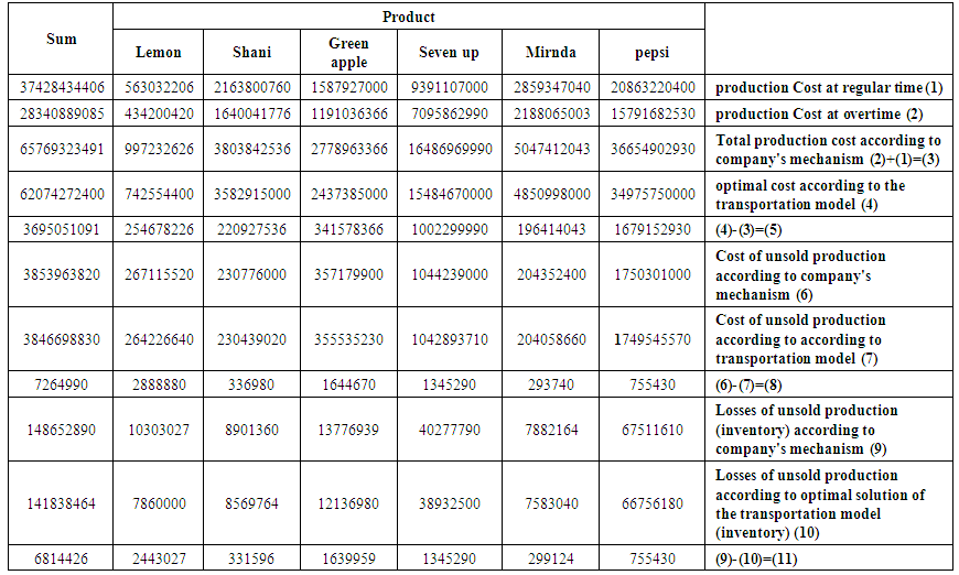 | Table (3). Production costs and losses according to company's mechanism and to the transportation model (in Iraqi dinar) |
For example, from the seven up transportation table, the quantities of unsold containers of production are 1053.64, 431.26, 3.44 and 3.43 respectively of production in the overtime of the first, second, third and fourth production periods, these quantities are multiplied by the corresponding storage cost, we will get the unsold production losses for seven up product according to the optimal solution of the transportation model,1053.64 (27000) +431.26 (24000) +3.44 (21000) +3.43 (18000) = 38932500 Iraqi dinars.We note that the unsold production losses of the seven up product according to the optimal solution of the transportation model are less than the unsold production losses according to company's mechanism. The difference is, 40277790-38932500 = 1345290 Iraqi dinars. These differences are positive for all products and then for their sum. Row 11 in table (3) contains these differences.4. Our main goal has been achieved, based on all of the above, Baghdad Soft Drinks Company can adopt the aggregate plan of production in Table (4) for all products under consideration (Pepsi, Miranda, Seven up, Green Apple, Shani, Lemon) and then their sum.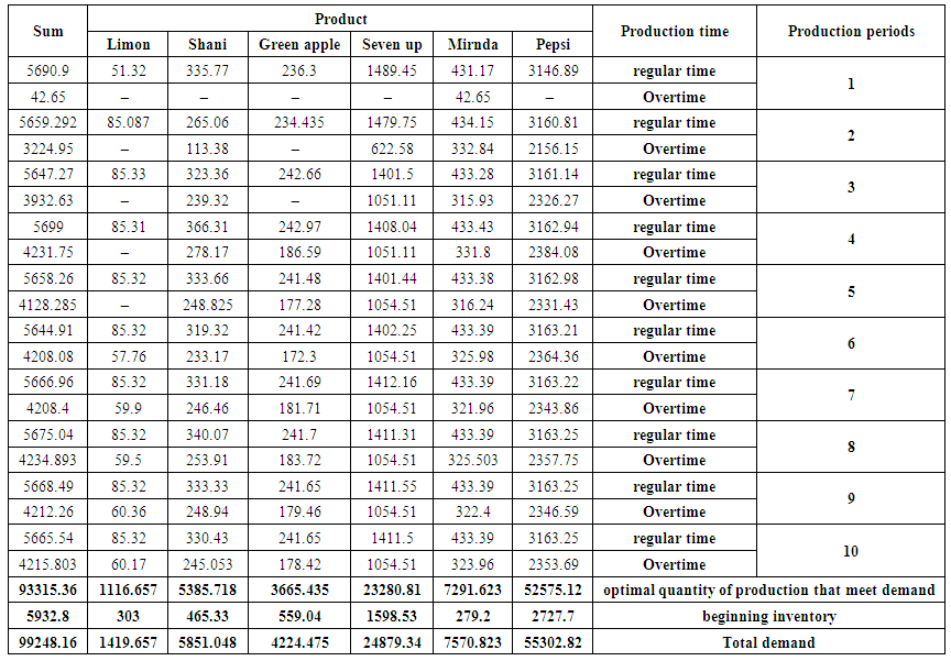 | Table (4). The optimal aggregate production plan for the months from March to December 2018 |
4. Conclusions, Recommendations and Future Studies
Before stating the conclusions, it should be stated that,1. The company is not designed an aggregate production plan but it is put an estimated annual plan in the light of achieved actual sales by using the method of the seasonal exponential smoothing, which is one of the simple forecasting methods. This plan is adopted for production purposes.2. The company did not specify the quantities of production in the regular time and the overtime required to meet the demand but the company adopted the method of production and storage directly, this leads to increase costs because of most of inventory production will be from production in overtime, without taking into account that need to meet the most demand from production in the regular time, while the remaining demand will be met from the production in overtime. This mean that the inventory at the end of the plan period must be zero or at least close to zero in the optimal aggregate production planning.3. The company did not specify from which Production batches (periods) should meet the sequential monthly demand so that costs are as low as possible.4. The company bears a cost of storage higher than the cost of the best plan (which is supposed to bear), since the unsold production was used as a beginning inventory in the beginning of the year.Then, an aggregate total production plan for all the studied products (Pepsi Cola, Miranda, Green apple, Seven up, Shani and Limon) has been putted, and thus for their total sum of 250ml metal cans category, in both regular time and overtime. production in 2018 under this plan fully covers the forecasted demand, taking into consideration the beginning inventory, since, it is well known that production is as much as demand in an optimal aggregate production plan. Some of the results of this optimal plan are as follows, 1. The total cost of production under the company's mechanism for each product and then for the total sum is greater than the cost reached according to the optimal solution of the transportation model.2. The cost of unsold production under the company's mechanism for each product and then for the total sum is greater than the unsold production cost reached according to the optimal solution of the transportation model.3. Losses of unsold production (inventory) according to the company's mechanism for each product and then for the total sum is greater than the losses of unsold production according to the optimal solution of transportation model.Based on the above, the bottom-up approach was used to assemble the plans of the six products under consideration to put the aggregate production plan. So, we are highly recommended to work according to the proposed optimal aggregate production plan.As future studies, we suggest using the optimization models along with an appropriate forecasting models to put an aggregate production plan for other families of products in Baghdad Soft Drinks Company and for other commodity products of other companies, also for services sector such as the health sector or Municipal sector. Also, we suggest studying the relationship between the use of transportation model to plan an aggregate production and achieve competitive dimensions.
Appendix
 | Table (1). Actual demand on produced containers for products under study |
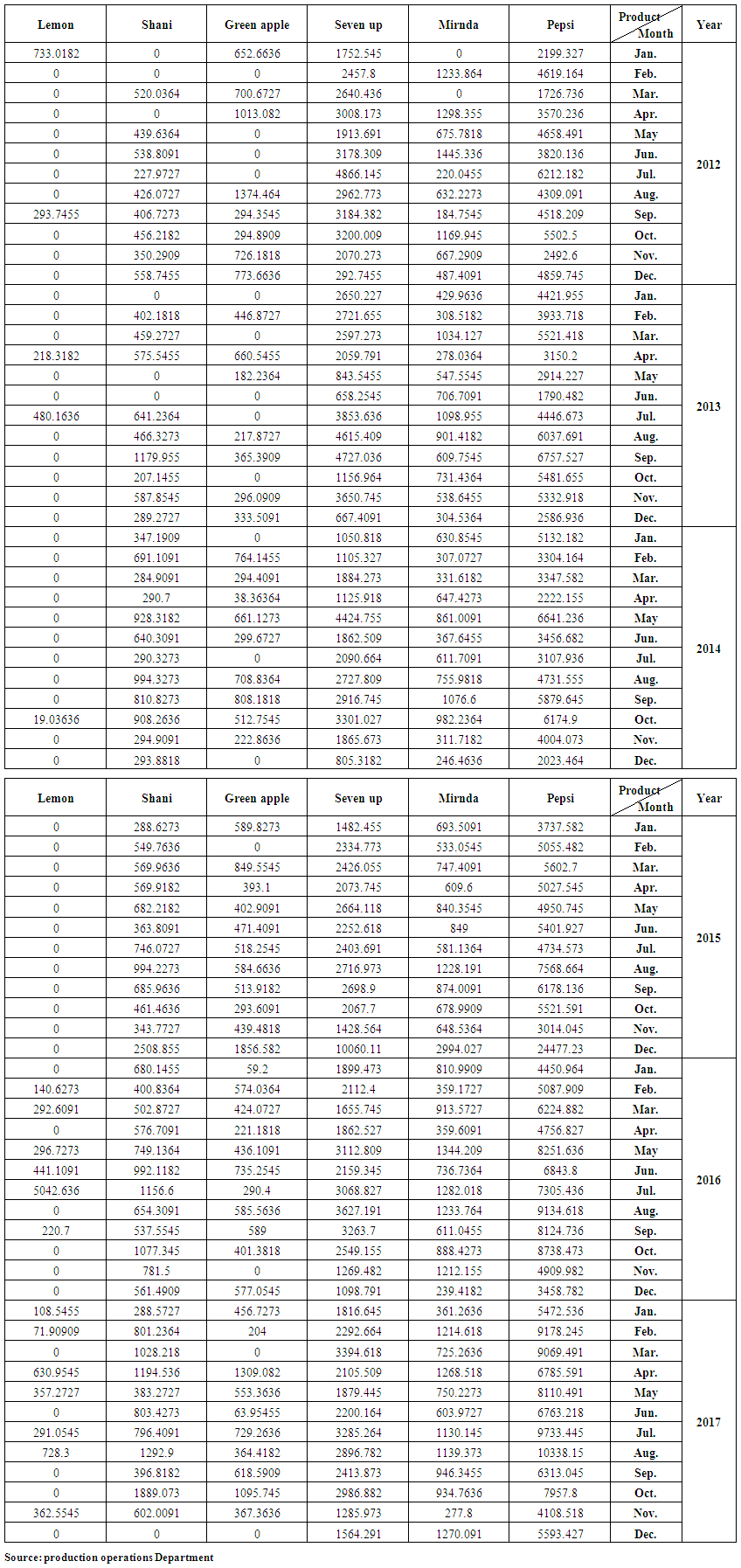 | Table (2). Actual production for produced containers |
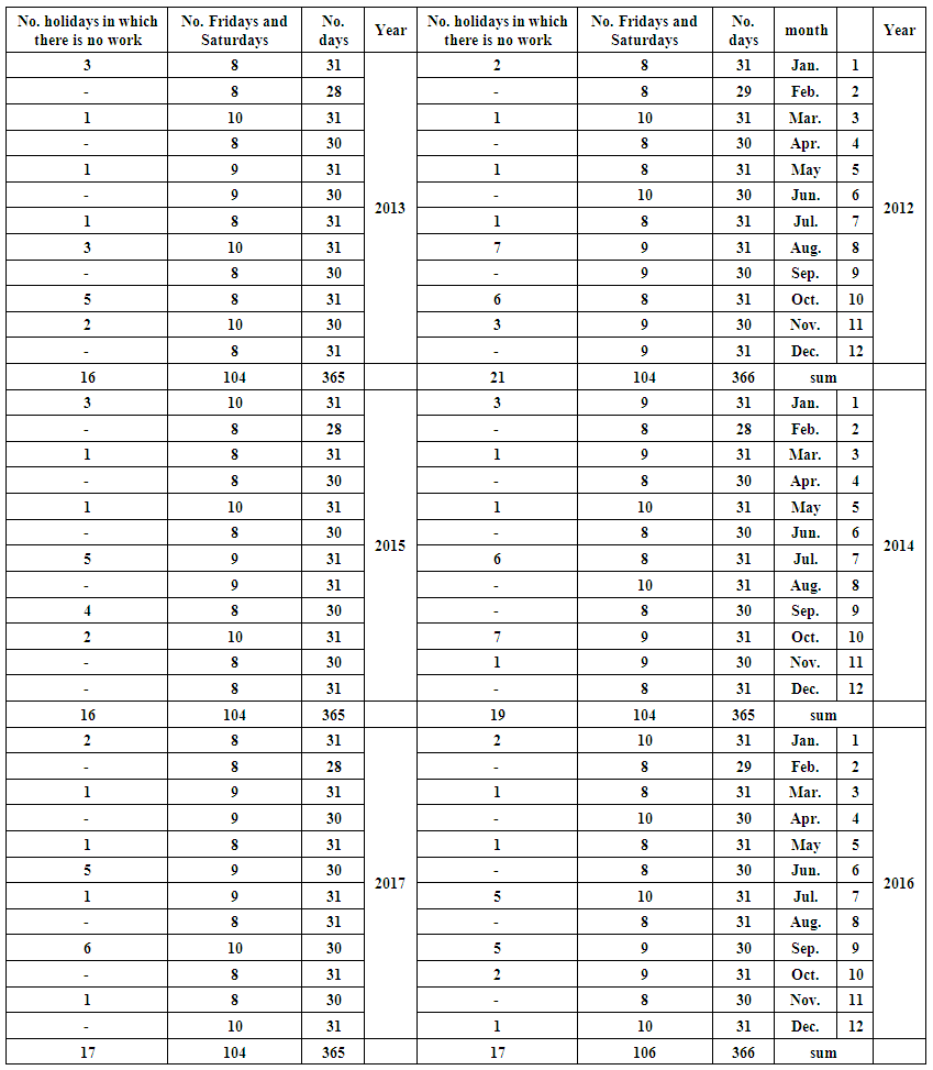 | Table (3). Public holidays over the period studied 2012-2017 |
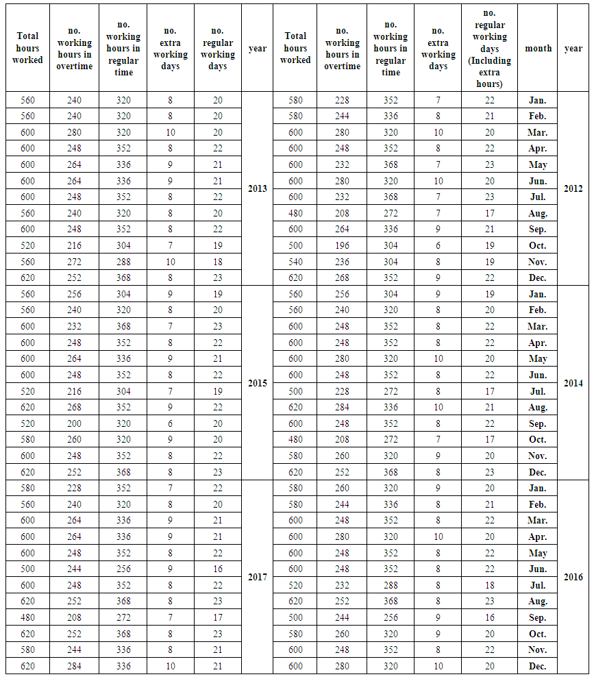 | Table (4). The number of hours worked at regular time and overtime |
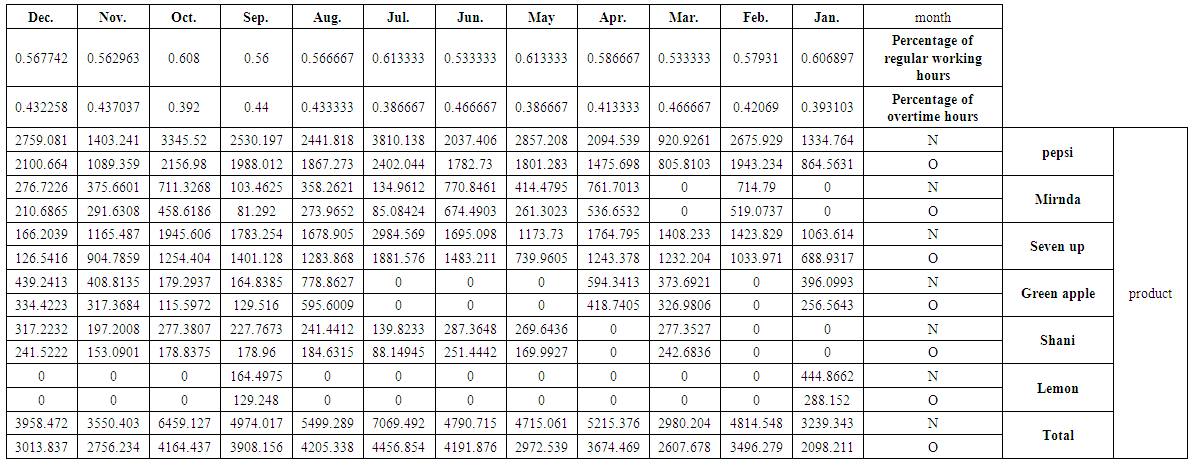 | Table (5). The quantity of production (s) at regular time N and overtime O for studied products and their total by the months for 2012 |
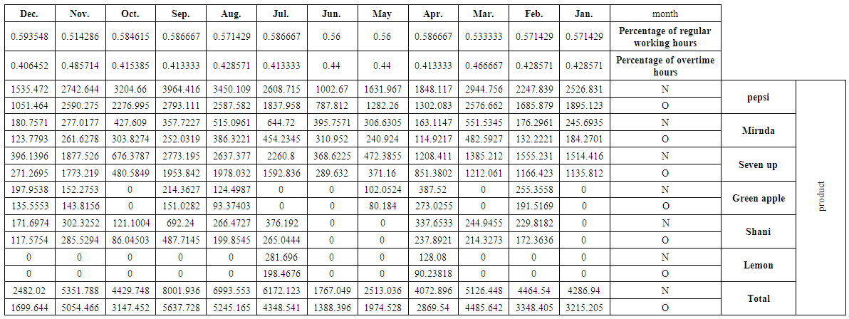 | Table (6). The quantity of production (s) at regular time N and overtime O for studied products and their total by the months for 2013 |
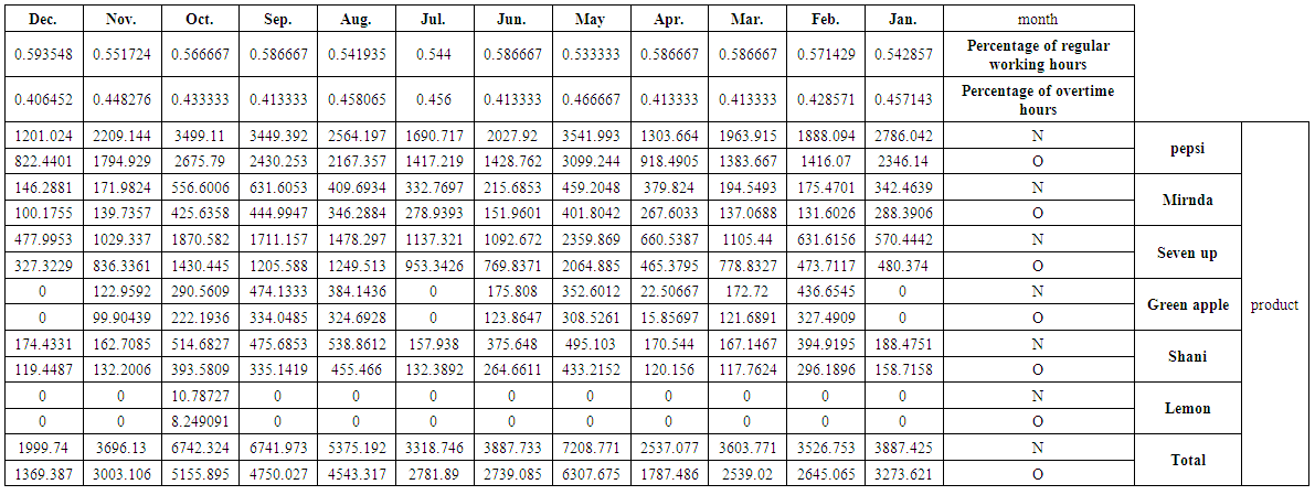 | Table (7). The quantity of production (s) at regular time N and overtime O for studied products and their total by the months for 2014 |
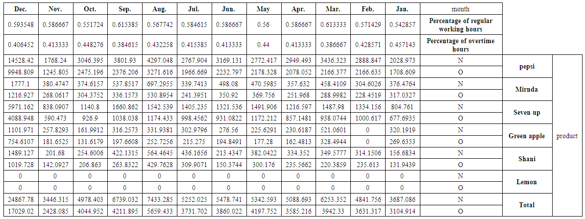 | Table (8). The quantity of production (s) at regular time N and overtime O for studied products and their total by the months for 2015 |
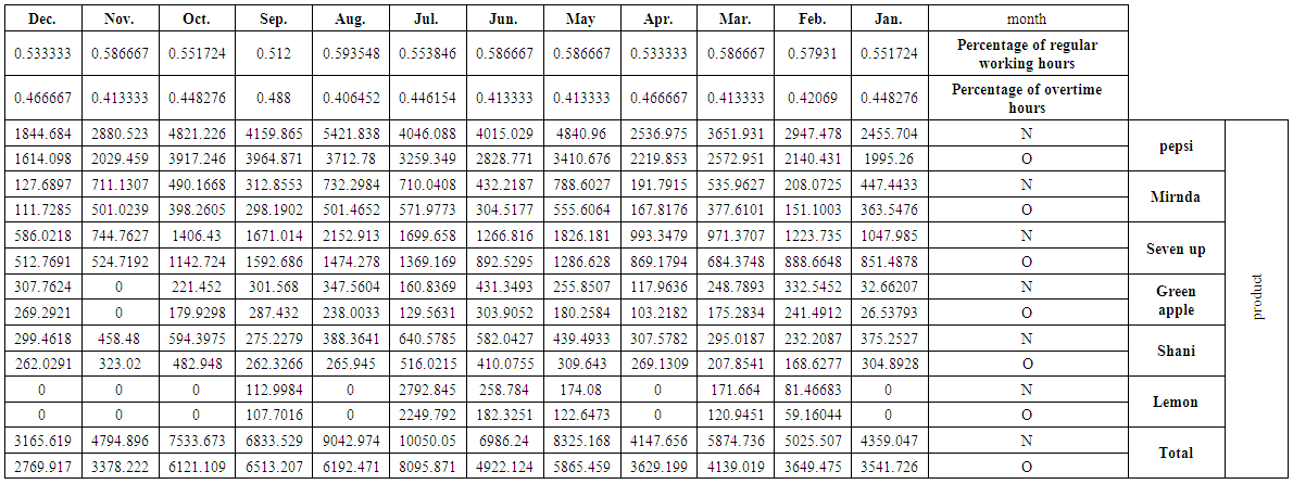 | Table (9). The quantity of production (s) at regular time N and overtime O for studied products and their total by the months for 2016 |
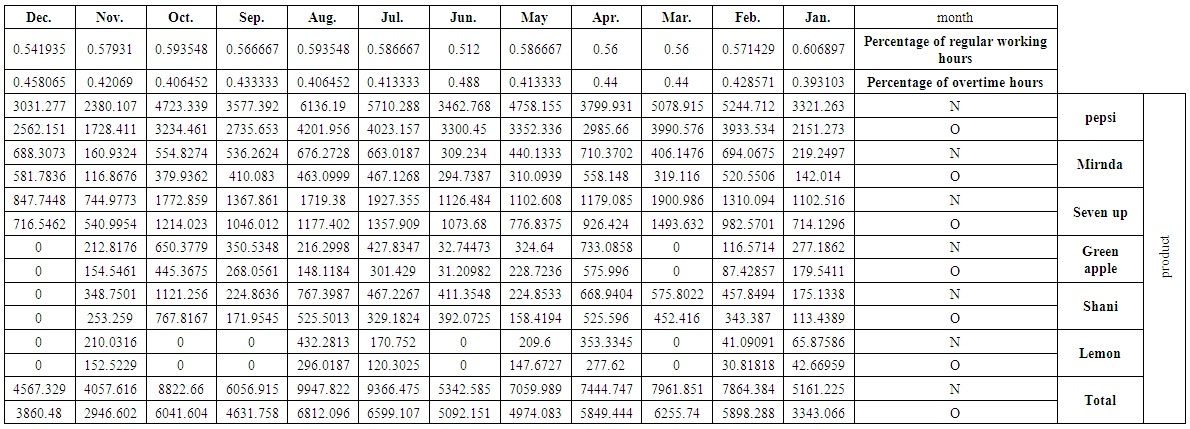 | Table (10). The quantity of production (s) at regular time N and overtime O for studied products and their total by the months 2017 |
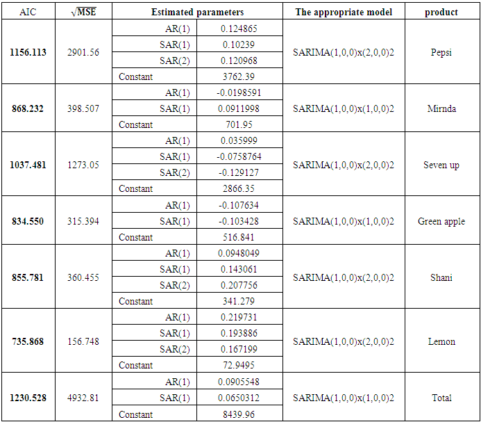 | Table (11). Statistical models used to represent the demand and forecast its future values for each product |
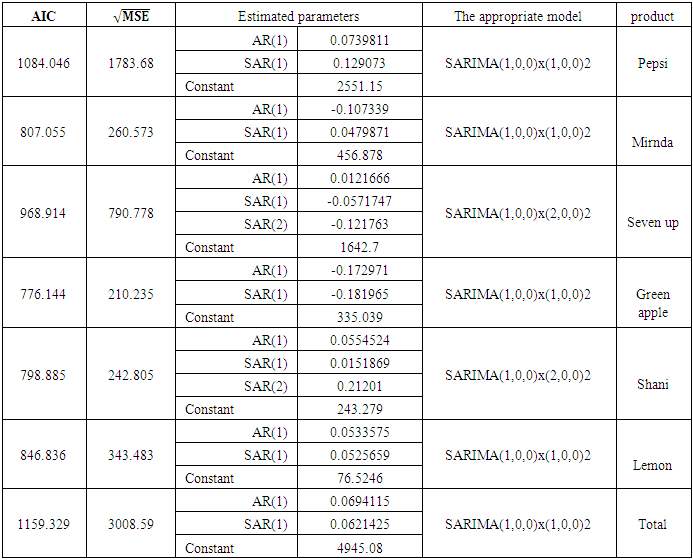 | Table (12). Statistical models used to represent the production in regular time and forecast its future values for each product |
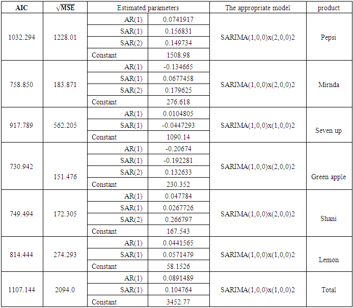 | Table (13). Statistical models used to represent the production in overtime and forecast its future values for each product |
 | Table (14). Results of the Box-Pierce statistic to check demand models ability for forecasting |
 | Table (15). Results of the Box-Pierce statistic to check ability of production models at regular time for forecasting |
 | Table (16). Results of the Box-Pierce statistic to check ability of production models at overtime for forecasting |
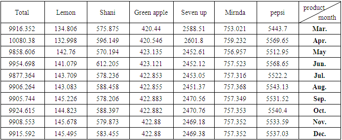 | Table (17). Forecasts of Demand for Months of 2018 from March to December for products under study and their total |
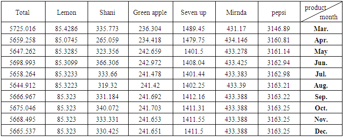 | Table (18). Forecasts of production at regular time for Months of 2018 from March to December for products under study and their total |
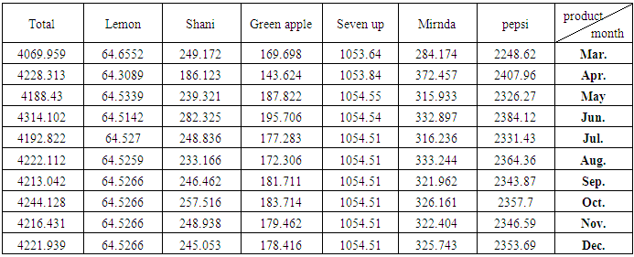 | Table (19). Forecasts of production at overtime for Months of 2018 from March to December for products under study and their total |
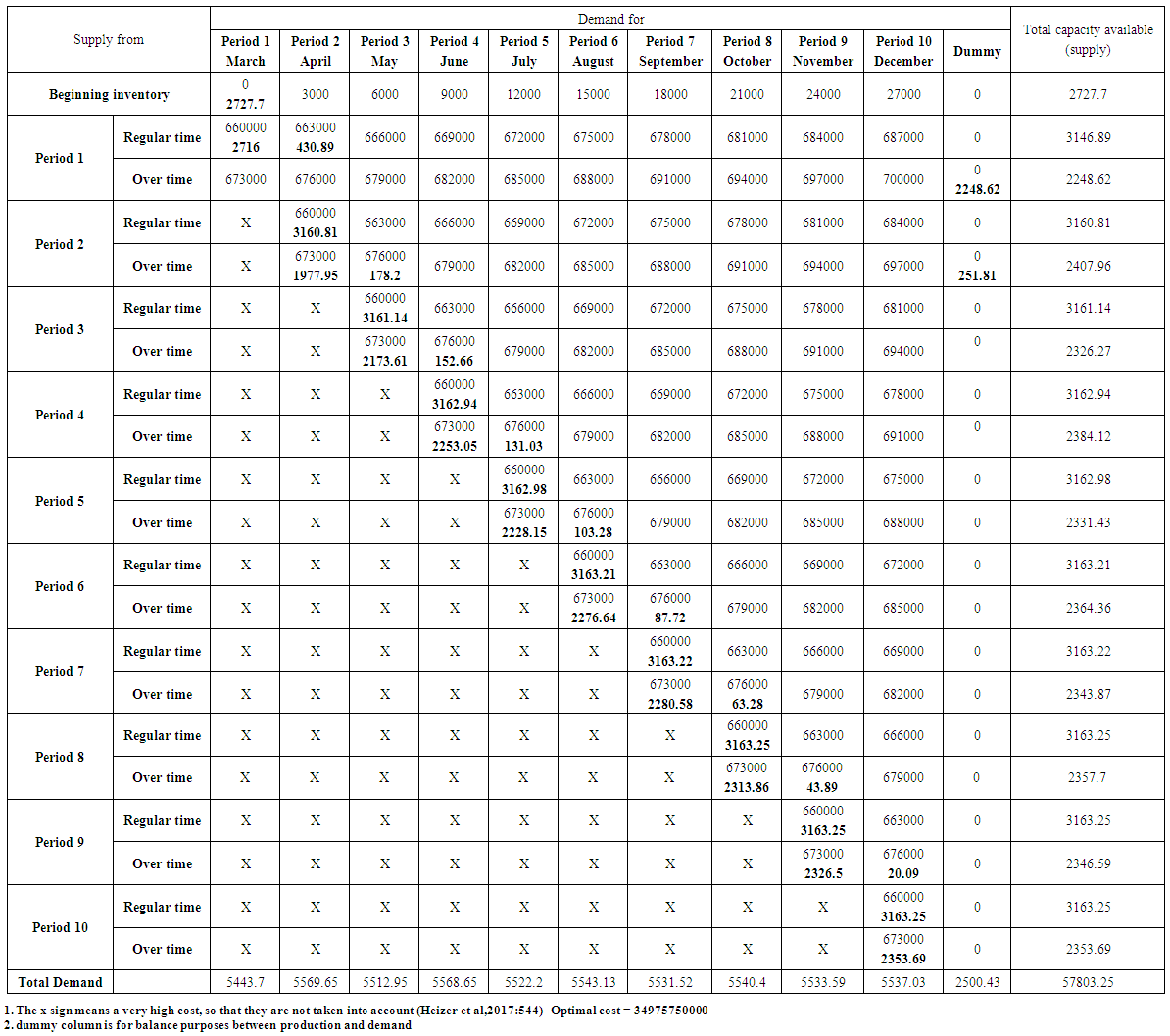 | Table (20). The optimal solution (lowest possible cost) using the transportation model for Pepsi product |
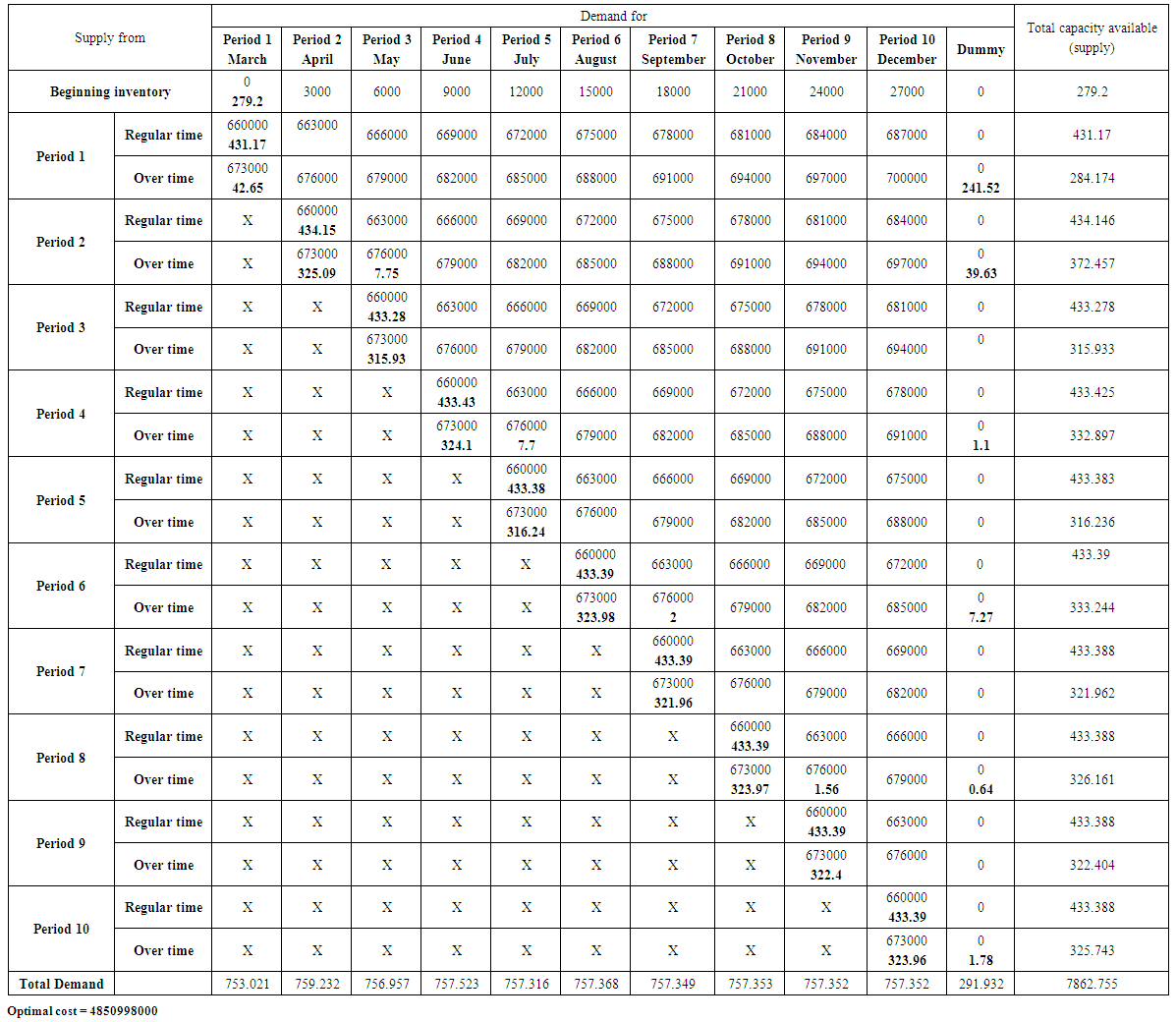 | Table (21). The optimal solution (lowest possible cost) using the transportation model for Mirnda product |
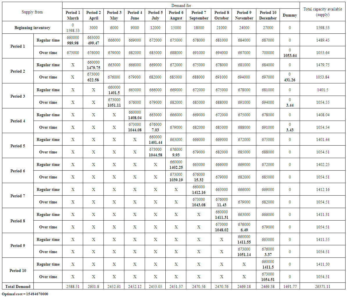 | Table (22). The optimal solution (lowest possible cost) using the transportation model for Seven up product |
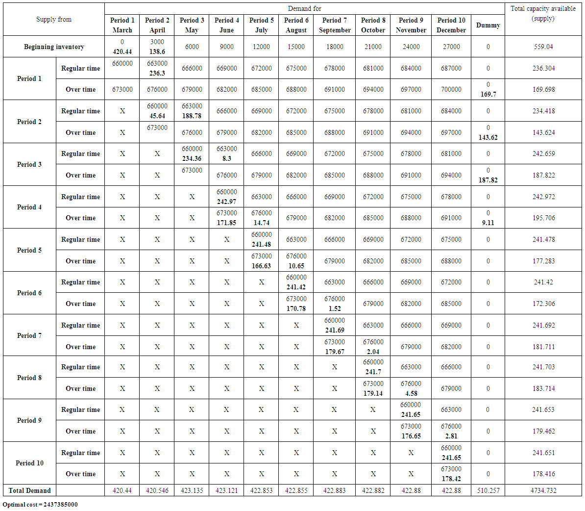 | Table (23). The optimal solution (lowest possible cost) using the transportation model for Green apple product |
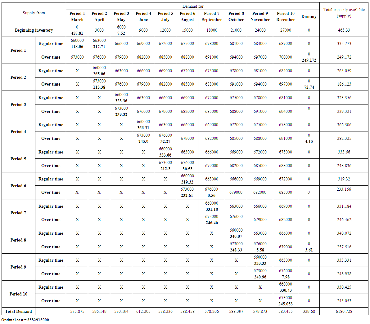 | Table (24). The optimal solution (lowest possible cost) using the transportation model for Shani product |
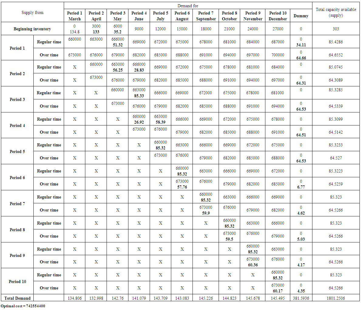 | Table (25) |
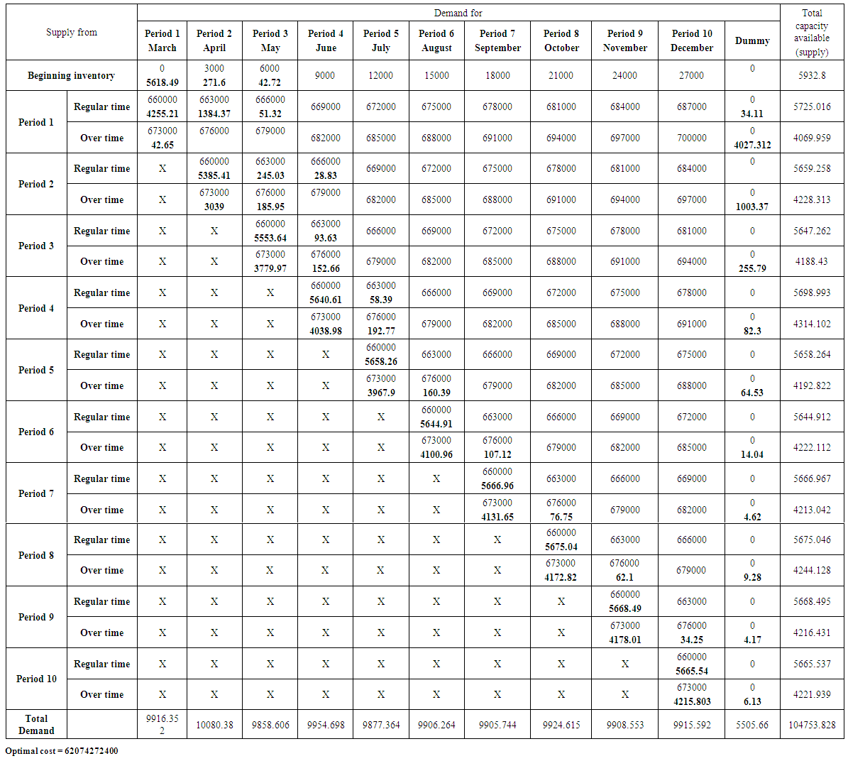 | Table (26). The optimal solution (lowest possible cost) using the transportation model for Total product |
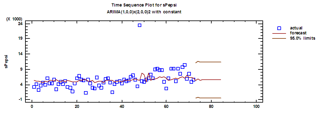 | Figure (1). Actual demand series on Pepsi and forecasts for 2018 |
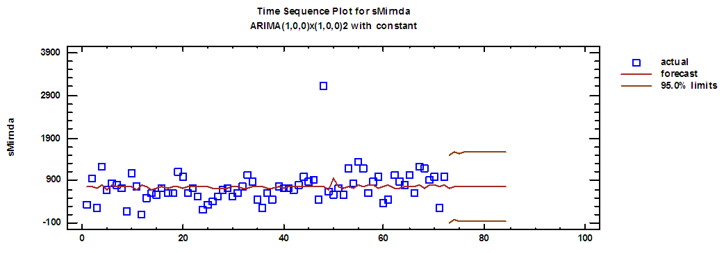 | Figure (2). Actual demand series on Mirnda and forecasts for 2018 |
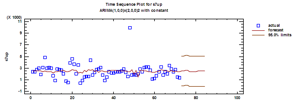 | Figure (3). Actual demand series on Seven up and forecasts for 2018 |
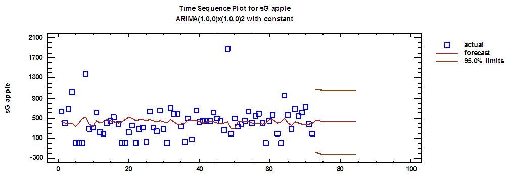 | Figure (4). Actual demand series on Green apple and forecasts for 2018 |
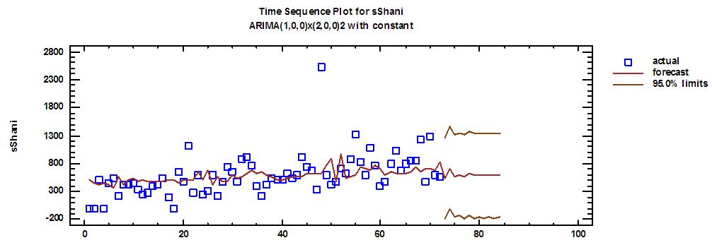 | Figure (5). Actual demand series on Shani and forecasts for 2018 |
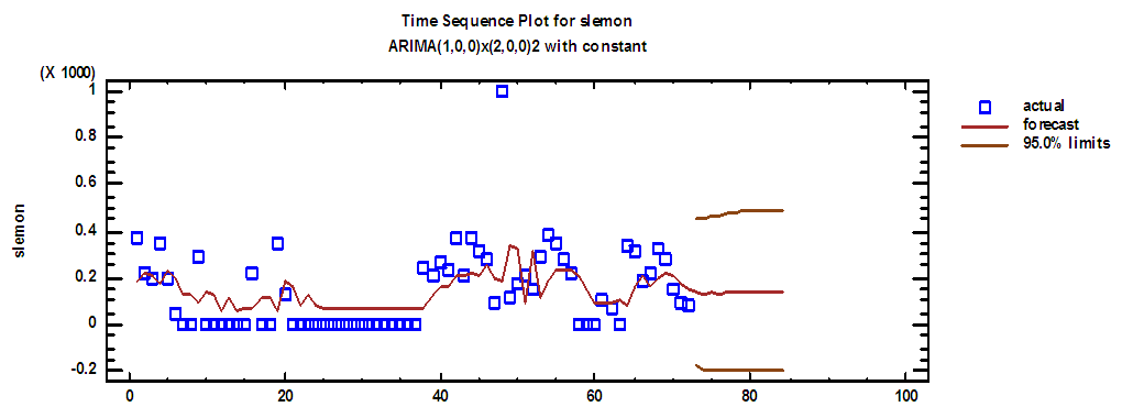 | Figure (6). Actual demand series on Lemon and forecasts for 2018 |
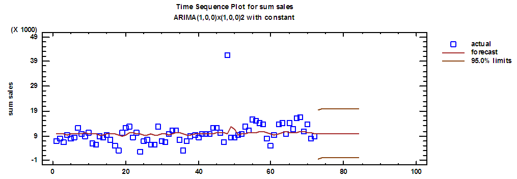 | Figure (7). Total actual demand series and forecasts for 2018 |
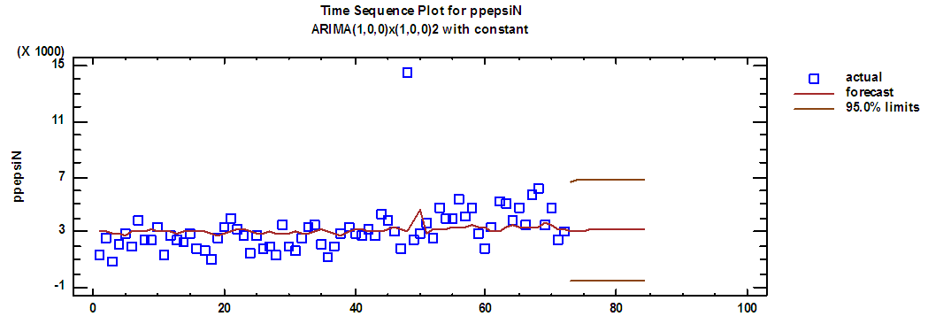 | Figure (8). Pepsi production series and forecasts for 2018 in regular time |
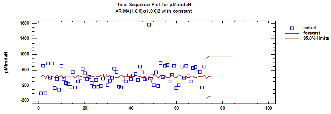 | Figure (9). Mirnda production series and forecasts for 2018 in regular time |
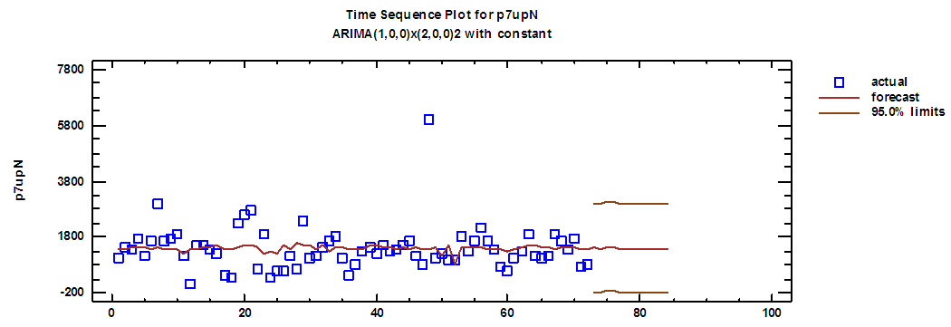 | Figure (10). Seven up production series and forecasts for 2018 in regular time |
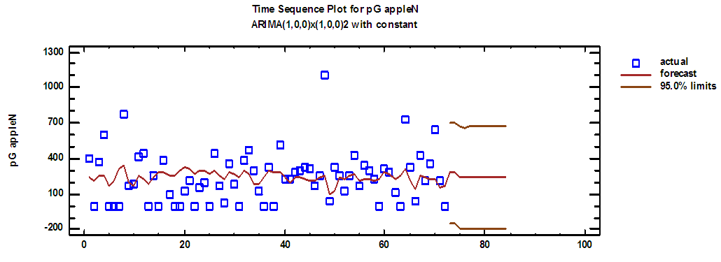 | Figure (11). Green apple production series and forecasts for 2018 in regular time |
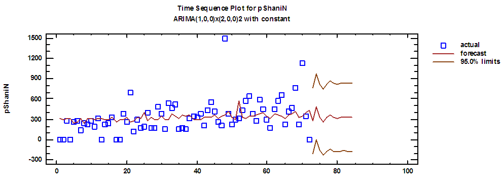 | Figure (12). Shani production series and forecasts for 2018 in regular time |
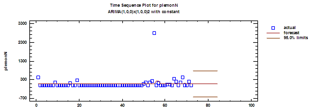 | Figure (13). Lemon production series and forecasts for 2018 in regular time |
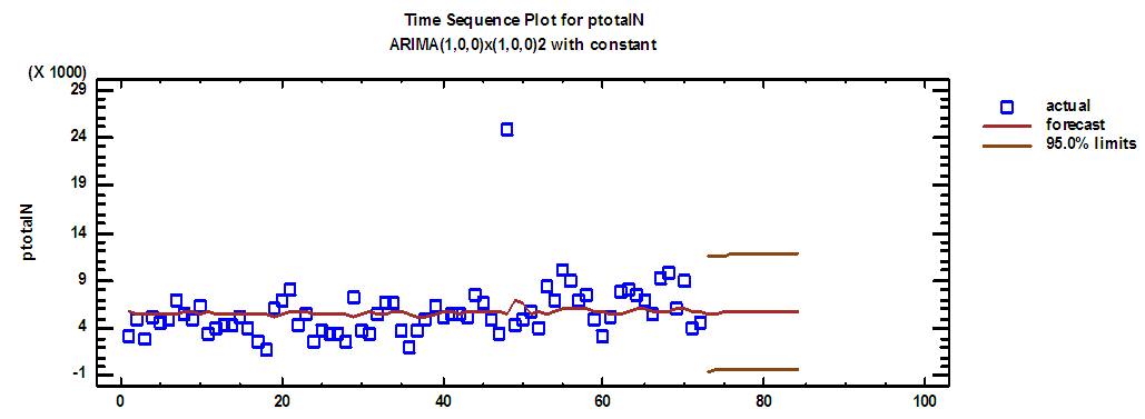 | Figure (14). Total production series and forecasts for 2018 in regular time |
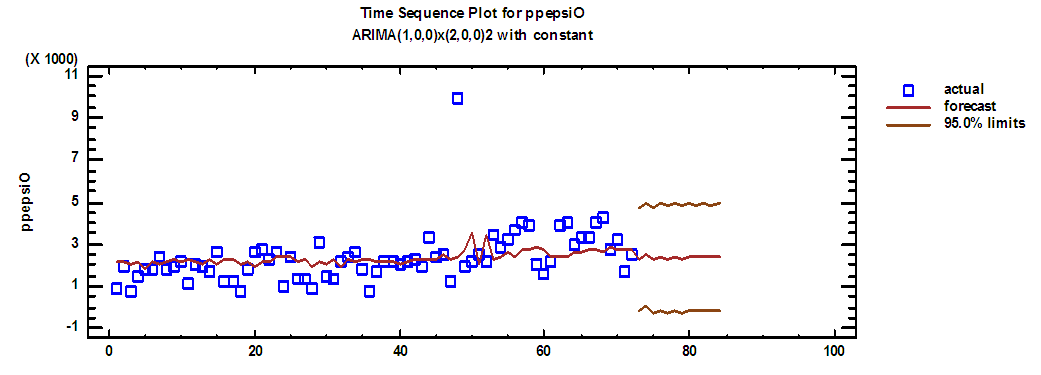 | Figure (15). Pepsi production series and forecasts for 2018 in overtime |
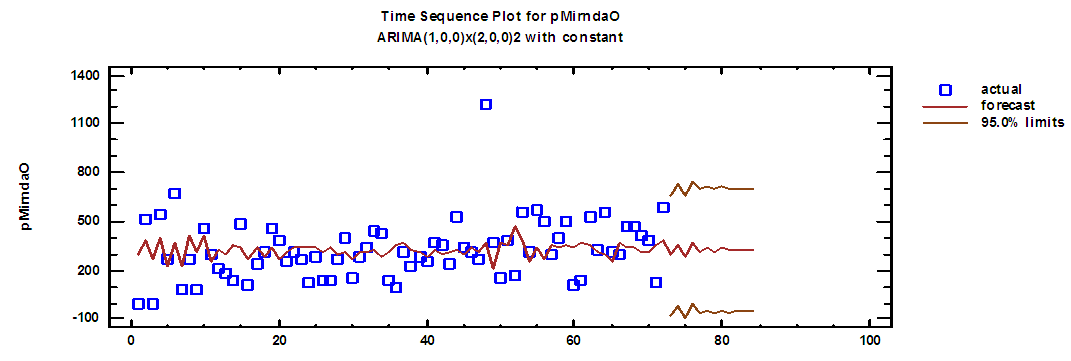 | Figure (16). Mirnda production series and forecasts for 2018 in overtime |
 | Figure (17). Seven up production series and forecasts for 2018 in overtime |
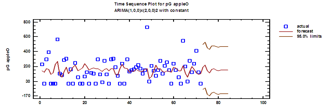 | Figure (18). Green apple production series and forecasts for 2018 in overtime |
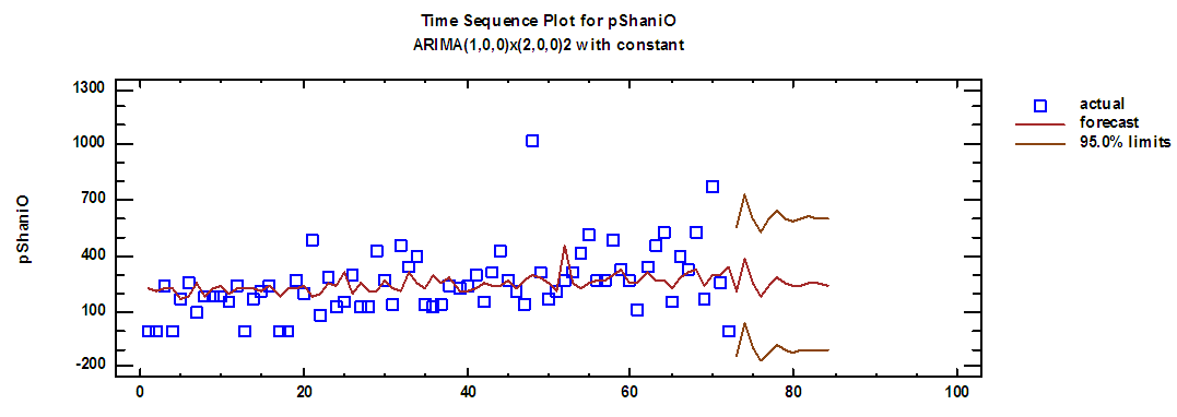 | Figure (19). Shani production series and forecasts for 2018 in overtime |
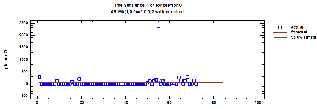 | Figure (20). Lemon production series and forecasts for 2018 in overtime |
 | Figure (21). Total production series and forecasts for 2018 in overtime |
References
| [1] | Box, G. Jenkins G. Reinsel, G. & Ljung, G. (2015), Time Series Analysis: Forecasting and Control, 5th ed, John Wiley & Sons, Ltd, USA. |
| [2] | Chada, C. (2015). Decision Support System in Aggregate Planning, Thesis for the Degree of Master of Science in Industrial Engineering, West Virginia University. |
| [3] | Damghani, K. Shahrokh, A. & Pakgohar, A. (2017) Stochastic multi-period multi-product multi-objective Aggregate Production Planning model in multi-echelon supply chain, International Journal of Production Management and Engineering, Vol. 5, No. 2, PP: 85-106. |
| [4] | Heizer, J. Render, B. & Munson, C. (2017), Operatians management: Sustainability and Supply Chain Management, 12th ed, Pearson Education, USA. |
| [5] | Jamalnia A. Yang, J. Ling, D & Feili, A, (2017), Novel decision model based on mixed chase and level strategy for aggregate production planning under uncertainty: Case study in beverage industry, Elsevier, International Journal of Production economics, Vol. 114, No. 2, PP 54-68. |
| [6] | Krajewski, L. & Ritzman, L. (2016), Operations management: Processes and Supply Chains, 7th ed, Courier Kendallville, USA. |
| [7] | Rosemary, E. & Edith, N. (2016), Transportation model: A qualitative solution tool for achieving institutional and managerial goals in the 21ST century, International Journal of Quantitative and Qualitative Research Methods, Vol. 4, No. 2, PP 1-9. |
| [8] | Stevenson, W. (2018), Operations Management, 13th ed, McGraw-Hill, NY. |
| [9] | Sultana, M. Shohan, S. Sufian, F. (2014), Aggregate planning using TransportatIon method, International Journal of Managing Value and Supply Chains (IJMVSC), Vol. 5, No. 3, PP 19 – 35. |
| [10] | Taha, H. (2016), Operation Research: An Introduction, 5th ed, Prentice Hall, PTR, NY, USA. |


 mathematically the ARIMA seasonal model is written as,
 and e represents a random error term.
 with constraints,

 There are some assumptions in the transportation model, that are, total quantity of the item available at different sources is equal to the total requirement at different destinations, item can be transported conveniently from all sources to destinations, the unit transportation cost of the item of the item from all sources to destinations is certainly and precisely known, the transportation cost on a given route is directly proportional to the number of units shipped on that route and the objective is to minimize the total transportation cost.The first step to solve transportation problem is to find out the initial feasible solution. The Vogel approximation method (VAM) is an iterative procedure for computing that basic feasible solution. This method is preferred over the other methods, because the initial basic feasible solution obtained by this method is either optimal or very close to the optimal solution. The steps in VAM are as follows, 1. Identify the boxes having minimum and next to minimum transportation cost in each row and write the difference (penalty) along the side of the table against the corresponding row.2. Identify the boxes having minimum and next to minimum transportation cost in each column and write the difference (penalty) against the corresponding column3. Identify the maximum penalty. If it is along the side of the table, make maximum allotment to the box having minimum cost of transportation in that row. If it is below the table, make maximum allotment to the box having minimum cost of transportation in that column.4. If the penalties corresponding to two or more rows or columns are equal, you are at liberty to break the tie arbitrarily.5. Repeat the above steps until all restrictions are satisfied.After computing an initial basic feasible solution, one can used the modified distribution method (MODI) is for finding the optimal solution of a transportation problem. It is provides a minimum cost solution. The steps in MODI are as follows,1. Determine the values of dual variables, ui and vj, using ui + vj = cij 2. Compute the opportunity cost using cij – ( ui + vj ). 3. Check the sign of each opportunity cost. If the opportunity costs of all the unoccupied cells are either positive or zero, the given solution is the optimal solution. On the other hand, if one or more unoccupied cell has negative opportunity cost, the given solution is not an optimal solution and further savings in transportation cost are possible. 4. Select the unoccupied cell with the smallest negative opportunity cost as the cell to be included in the next solution. 6. Draw a closed path or loop for the unoccupied cell selected in the previous step. Please note that the right angle turn in this path is permitted only at occupied cells and at the original unoccupied cell. 7. Assign alternate plus and minus signs at the unoccupied cells on the corner points of the closed path with a plus sign at the cell being evaluated. 8. Determine the maximum number of units that should be shipped to this unoccupied cell. The smallest value with a negative position on the closed path indicates the number of units that can be shipped to the entering cell. Now, add this quantity to all the cells on the corner points of the closed path marked with plus signs, and subtract it from those cells marked with minus signs. In this way, an unoccupied cell becomes an occupied cell.
 is used to determine the advantage of a model among several models were estimated.a. The models mentioned in Table (11) In annex, are appropriate to represent the demand on containers for each product, and then the total demand for the sum of all products.b. The models mentioned in Table (12) In annex, are appropriate to represent quantities of production on containers for each product within the regular time, and then the total quantities of production for the sum of all products.c. The models mentioned in Table (13) In annex, are appropriate to represent quantities of production on containers for each product within the overtime, and then the total quantities of production for the sum of all products.It should be noted that the criterion for selecting the appropriate model is the least value of √MSE and the lowest value of the AIC criterion, for example SARIMA (1.0,0) x (2,0,0) 2, is a model which was chosen to represent demand. It was used to forecast future values for Pepsi, with value of √MSE equal to 2901.56 and value of Akiaki criterion equal to 1156.113, which are the lowest among all corresponding values of the models selected to represent the demand for Pepsi product.SARIMA (1,0,0) x (2.0.0) 2 model, which is represented the demand on the Pepsi, can be written according to the equation (1) as follows,

 Equation (2) will be:


 Abstract
 Reference
 Full-Text PDF
 Full-text HTML