1. Introduction

A developer that owns a shopping center (SC) closes tenants’ lease contracts with retailers. In particular, for apparel companies, having larger stores tenanted in an SC makes it possible to provide consumers with better services by offering a wide product assortment and hiring more staff who engage in service provision in the store. Therefore, the size of store space for retailers is a major factor that determines the quality of their services and therefore their profit. Thus, when more space is allocated to a retailer by the developer, the increase in space allocation boosts the profit of the retailer. Moreover, space allocation in an SC is also an important issue for the developer since it determines its profit. While the efficiency of retailers varies significantly in reality, we categorize retailers into two types of companies for the tractability of our model: efficient and inefficient companies. The former includes dominant retailers (e.g., ZARA, H&M, UNIQLO) and all the other companies are categorized as weak retailers.

Favorable contracts are applied in some types of apparel retailing. By considering space allocation in an SC in particular, we discuss whether developers allocate more space to dominant retailers. Previous studies have also examined this problem and discussed favorable contracts that involve rents imposed on retailers (Benjamin and Chinloy 2004; Brueckner 1993; Cho and Shilling 2007; Colwell and Munneke 1998; Gerbich 1998; Gould et al. 2005; Pashigian and Gould 1998; Wheaton 2000) and space allocation (Benjamin et al. 1990, 1992; Brueckner 1993; Eppli and Benjamin 1994; Gerbich 1998; Gould et al. 2005; Miceli et al. 1998; Mooradian and Yang 2000; Wheaton 2000). A developer offers a favorable contract (e.g., more space and/or lower rent) to dominant retailers based on their strong bargaining power and positive externalities (Brueckner 1993; Cho and Shilling 2007; Eppli and Benjamin 1994; Gould et al. 2005; Miceli et al. 1998). In this case, the space allocation and profit of a developer may have a negative correlation because the developer faces unfavorable contracts with dominant retailers. However, such a phenomenon includes the two effects of space allocation and rent reduction, which should be distinguished.

Therefore, in this paper we focus only on the space allocation effect by assuming that the rent for a dominant retailer is an exogenous fixed rental rate. The assumption of a fixed rent is also used in the model of Geylani et al. (2007). The interpretation of this assumption is that developers close contracts with dominant retailers that feature extremely low rental rates since dominant retailers have stronger bargaining power, which lends them an advantage during negotiations and positive externalities in an SC. The developers in this model consider how to allocate space to dominant retailers that yield little profit from the rental.

We consider a vertical relationship between a developer and two asymmetric types of retailers in an SC, namely a dominant retailer and a weak retailer. The timing of our model is as follows. First, the developer allocates space to both retailers and decides the rent for the weak retailer (recall that the rental rate for the dominant retailer is fixed). Second, the sales quantity of each retailer is determined.

Tenant contracts in SCs have two types of rental payments: pay a fixed rent for a certain period of time or pay depending on sales volume. An example of the latter agreement is a percentage rent (Benjamin and Chinloy 2004; Cho and Shilling 2007; Chun et al. 2001; François et al. 2005; Gould et al. 2005; Mooradian and Yang 2000; Colwell and Munneke 1998; Wheaton 2000). We assume that the rent depends on the volume of sales in our model. Moreover, we provide a game-theoretic model to discuss the relationship between space allocation to each retailer and the profit of a developer. In the model, a developer unilaterally allocates space when the rental rate for a dominant retailer is fixed at some exogenously determined small rate.

Apparently, a developer may increase its profit by allocating more space to a dominant retailer; that is, the relation between the space of a dominant retailer and the developer’s profit may be positive. However, the analysis in this paper shows that these variables have a negative relation in the equilibrium. The factor leading to such a result is dependent on the decrease in the sales promotion cost for a weak retailer. A developer determines space allocation by taking into account the sales promotion cost for both types of retailers and the rent incurred by them. Since a dominant retailer can decrease the sales promotion cost, which makes it relatively efficient, it would be advantageous for a developer to allocate more space to a dominant retailer. On the contrary, although a weak retailer must pay a higher sales promotion cost in the equilibrium, the developer assists the weak retailer by decreasing its rent. As a result, the developer decreases its profit. That is, we find that the total sales promotion cost of all SCs increases in the equilibrium. These aspects have not been focused upon in previous studies (Brueckner 1993; Cho and Shilling 2007; Eppli and Benjamin 1994; Gould et al. 2005; Miceli et al. 1998).

The remainder of this paper proceeds as follows. The next section presents the model. Section 3 calculates the equilibrium and provides the main results. Section 4 concludes the paper.

2. The Model

We assume an SC where a developer determines the space allocated to two types of retailers. To sell products, each retailer must sign lease contracts with the developer. We call the retailer with higher efficiency the dominant retailer (DR) and the other with lower efficiency the weak retailer (WR). We assume that the dominant retailer’s marginal cost, except purchasing expenses and the cost of rent, is normalized to zero, while that of the weak retailer is and the cost of purchase is w. We assume that w is zero because the retailers get the product from manufacturers except developer. Then, we assume a cost-competitive setting such as that in the apparel industry. We consider that each retailer’s rent depends on its sales 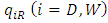. For simplicity, we assume that is the rent according to rental rate (unit rent) and amount of sales that retailer attains. The dominant retailer is assumed to be offered a more favorable contract with a relatively low rental rate which is close to zero. We interpret this assumption as a situation where the dominant retailer has good outside options (e.g., contracting with other SCs) and developers cannot renegotiate the rental rate with the dominant retailer. Thus, we assume that the unit rent of the dominant retailer is fixed as an exogenous parameter. In our model, the quality of the products sold by the retailers is composed of two elements, namely product quality and service quality. We assume that the product quality of the weak retailer denoted by is higher than that of the dominant retailer , while the marginal cost of the dominant retailer is lower than that of the weak retailer. Service quality depends on the size of each retailer’s space, which is determined by the developer. We denote the size of the space of retailer by .

The utility maximization problem is

(1)

where m is the amount of the numeraire good, is the price of retailer’s product, and is income for the consumer. We employ the utility function form represented by Equation (1) for the following reason. If either the product quality or the service quality supplied by a retailer is zero, a consumer has no incentive to buy the product. In our model, marginal utility is negative, , whenever one or both qualities are zero. Hence, our utility function is consistent with consumer behavior. Previous studies considering the space allocation problem use a similar form of utility function (Miceli et al. 1998).

Moreover, several previous studies interpret the intercept of an inverse demand function as the quality of the product (Häckner 2000; Rosenkranz 2003). To obtain clear results, we add the following assumptions for the utility function. We normalize the total space of SCs to 1 and define . In addition, we assume that and , since the product quality of the weak retailer is higher than that of the dominant retailer. From the first-order conditions of the utility maximization problem, the inverse demand functions that the two retailers face are given by

(2)

(3)

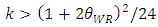
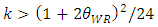
We assume that a developer has already designed the basic layout of the SC, which apportions space between the dominant retailer and weak retailer. Then, we call the space in the basic layout for one retailer and we assume the developer determines the layout of space for dominant retailer by less than 70% of the whole SC in consideration of actual space. Next, after the developer closes a contract with each retailer, which determines the space of each store, it changes the basic layout (e.g., aisles and walls), according to the partition between stores fixed by the contract. Therefore, the developer incurs more cost for remodeling the basic layout when one type of retailer acquires more space than the other. We assume that the parameter of the cost is k, which increases as the difference from the original layout grows. In addition, we assume sufficiently large k to eliminate the case when the developer cannot keep positive outcomes. To assure a unique maximum for and , which maximizes the profit functions of the developer, we assume that the profit function consequently is concave in and . Then, concavity implies that the Hessian matrix must be negative definite. By solving the determinant of the Hessian matrix, concavity implies that , which is also derived from (13), namely the second-order condition as the developer chooses the space of the dominant retailer.

The profit of the developer is

(4)

The profit of retailer is

(5)

(6)

The setting of the assumption and timing of the game are described as follows. First, given the unit rent of the dominant retailer , the developer chooses the size of the space for the retailers, and . At the same time, the developer chooses the unit rent imposed on the weak retailer, . Next, each retailer simultaneously chooses its sales, . The model is solved with the use of backward induction along the timeline to derive the subgame perfect equilibrium in this dynamic game.

3. Calculating Equilibrium

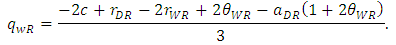
In this section, we identify the subgame perfect equilibrium. In the second stage, each retailer chooses its sales quantity.

The maximization problem for the dominant retailer is

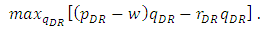(7)

The maximization problem for the weak retailer is stated as

(8)

The first-order conditions are derived as

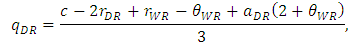(9)

(10)

By substituting this outcome into the profit of the developer, we have the maximization problem of the developer as follows:

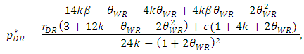
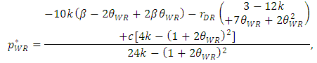
(11)

The first-order condition in this stage yields

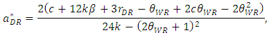(12)

(13)

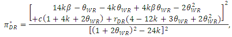
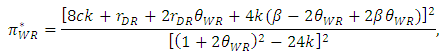
where the variables with superscript * represent the equilibrium values. Therefore, the second-order condition leads to the assumption , and the inequalities are satisfied. Substituting Equations (9), (10), (12), and (13) into Equations (2)–(6) gives the equilibrium profit as follows:

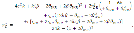(14)

(15)

(16)

(17)

(18)

(19)

(20)

By differentiating these equilibrium outcomes with respect to the marginal cost of the weak retailer c, we obtain the following proposition.

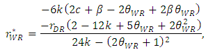
Proposition 1 As the sales promotion cost of the weak retailer c increases, the sales volume of the weak retailer decreases, the price of each retailer and increases, and the sales volume of the dominant retailer increases in the equilibrium. Then, the rent for the weak retailer and the profit of the developer decrease.

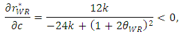(21)

(22)

(23)

(24)

(25)

(26)

(27)

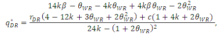
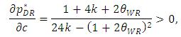
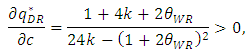
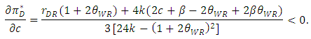
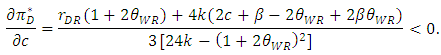
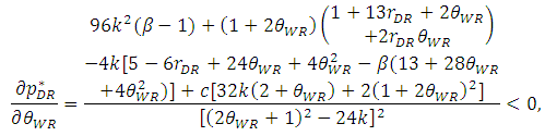
Proof. Given the assumption , the inequalities are satisfied.

From Proposition 1, when the sales promotion cost of the weak retailer increases, its sales volume decreases and its price increases in the equilibrium. Then, the developer assists the weak retailer by decreasing its rent. As a result, the developer decreases its profit. In general, the developer might widen the rent gap between the two types of retailers in such a situation since the weak retailer has no competitive advantage over the dominant retailer. However, we find that the developer assists the weak retailer by restraining the difference in the rent between both retailers in an SC. Moreover, we also find that the total sales promotion cost of the whole SC increases in the equilibrium as explained next.

Proposition 1 shows that as the marginal cost of the weak retailer c increases, the unit rent for the weak retailer decreases. Based on Proposition 1, we thus show that an increase in c raises the sum of the marginal cost plus the unit rent for the weak retailer .

By differentiating with respect to c, we have the following lemma.

Lemma 1 As the marginal cost of the weak retailer c increases, the total marginal cost increases. However, the decrease in the change in the unit rent is smaller than the increase in c.

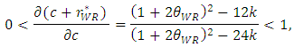(28)

Proof. Given the assumption , the inequalities are satisfied.

The intuition behind this lemma is as follows. Since an increase in the marginal cost of the weak retailer c decreases the degree of competition between the two retailers, the developer reduces the unit rent of the weak retailer to increase the competitiveness of the retail market. This adjustment cannot retrieve the former state. Then, the decrease in the unit rent of the weak retailer is smaller than the increase in the marginal cost of the weak retailer c.

In addition, we provide a detailed explanation of the intuition. From Proposition 1, the increase in the marginal cost of the weak retailer c decreases the unit rent for the weak retailer . Then, it is not clear whether the total marginal cost of the weak retailer increases. Hence, from Lemma 1, the increase in the marginal cost of the weak retailer c always increases the total marginal cost of the weak retailer in the equilibrium. Then, the increase in the marginal cost of the weak retailer c increases the sales promotion cost of the weak retailer. Therefore, the developer decreases the unit rent of the weak retailer to promote the relative competitiveness between the retailers. The degree of the decrease in the unit rent of the weak retailer is smaller than the degree of the increase in the marginal cost of the weak retailer c.

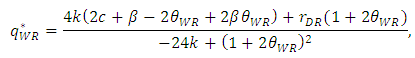
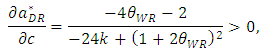
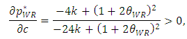
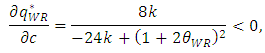
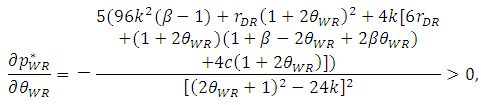
By differentiating and with respect to c, we have the following the lemma.

Lemma 2 As the marginal cost of the weak retailer c increases, space allocation to the dominant retailer increases and the profit of the developer decreases.

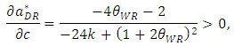(29)

(30)

Proof. Given the assumption , the inequalities are satisfied.

When the marginal cost of the weak retailer c increases, the dominant retailer decreases the sales promotion cost and becomes a relatively more efficient company. Therefore, the developer will expect to gain more profit when it allocates more space to the dominant retailer since the dominant retailer can promote sales at a lower cost. For the reasons stated above, the developer allocates more space to the dominant retailer . However, the developer decreases its own profit at the same time.

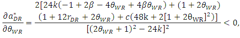
By differentiating these outcomes with respect to the product quality of the weak retailer , we obtain the following proposition.

Proposition 2 As the quality of the weak retailer , increases, the equilibrium of space allocation to the dominant retailer , the price of the dominant retailer , and the quantity of the dominant retailer decrease. As the quality of the weak retailer , increases, the equilibrium of the unit rent of the weak retailer , the price of the weak , and the quantity of the weak retailer increase.

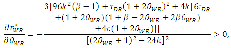(31)

(32)

(33)

(34)

(35)

(36)

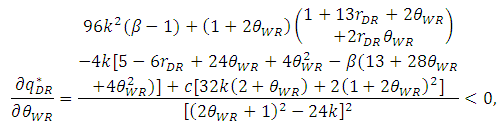
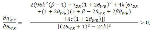
Proof. Given the assumption , the inequalities are satisfied.

From Proposition 2, the product quality of the weak retailer increases with the unit rent of the weak retailer . In this case, when the weak retailer can offer better goods to customers in small high brand retail stores, the developer gains more rent from the weak retailer. As the product quality of the weak retailer increases, space allocation to the dominant retailer decreases. When the weak retailer can offer good products, the developer allocates less space to the dominant retailer.

Then, as the product quality of the weak retailer increases, the price of the weak retailer increases. This situation is readily imagined and stands to reason. Since the quality of the weak retailer increases, the price of the weak retailer obviously increases. Then, an increase in the product quality of the weak retailer also decreases the price of the dominant retailer since the relative quality of the dominant retailer decreases.

Moreover, as the product quality of the weak retailer increases, the sales volume of the weak retailer increases even though the price of the weak retailer increases. An increase in the product quality of the weak retailer decreases the sales volume of the dominant retailer regardless of the decrease in the price of the dominant retailer. In general, although the relationship between the sales volume of the product and price has a negative correlation, in our model, it has a positive correlation between the volume of the product of the dominant retailer and the price of the dominant retailer.

The intuition behind parts of Proposition 2 is as follows. When the quality of the weak retailer increases, the developer allocates less space to the dominant retailer and the sales volume of the dominant retailer decreases even though the price of the dominant retailer decreases.

Next, we mention the difference in rent for the retailers in an SC. From Proposition 2, since an increase in the quality of the weak retailer increases the unit rent of the weak retailer , the difference in the rent between the dominant retailer and weak retailer in an SC is expanded by the quality of the weak retailer . Conversely, it is better to narrow the difference in the rent between the dominant retailer and weak retailer as the quality of the weak retailer approaches the quality of the dominant retailer.

In our model, we conclude that the developer should widen the gap in the rent between a dominant retailer and a weak retailer when a small specialized shop is offering high-value added brands. In general, a developer might not widen the gap in the rent between these two types of retailers in such a situation since the weak retailer has such a competitive advantage over the dominant retailer that the weak retailer has bargaining power to the developer, too. Therefore, although it may be considered that the developer will give preferential treatment to the weak retailer as well as to the dominant retailer, we find that the difference in the rent between both retailers in an SC should be expanded to raise the profit of the developer.

4. Conclusions

We provide a game-theoretic model to discuss the relationship between space allocation to retailers and the profit of the developer, assuming that two types of asymmetric retailers close contracts with a developer of SCs. The main findings of this research are summarized as follows.

We show that a developer allocates more space to a dominant retailer in the equilibrium even though the developer’s own profit falls. Under the circumstances where a developer unilaterally allocates the space of SCs, it may be imagined that it expects to increase its profit by allocating more space to the dominant retailer (i.e., the size of space and profit have a positive relationship). However, as we show, these variables have a negative relationship in the equilibrium in our model. In other words, we suspect that developers would face a dilemma about whether to allocate more space to dominant retailers in spite of decreasing their profit.

Moreover, we show that this situation leads to increasing the sales promotion cost for the weak retailer. Since an increase in the marginal cost of the weak retailer means a relative decrease in the cost of the dominant retailer, a developer allocates more space to the latter. Then, we conclude that an increase in the total sales promotion cost of SCs leads to a fall in the profit of the developer even though the dominant retailer can promote sales efficiently through its store image and advertisements. Furthermore, we also find that an increase in the marginal cost of the weak retailer increases the sales promotion cost of the overall SC, which decreases the profit of the developer. Then, the developer assists the weak retailer by decreasing its rent. As a result, the developer decreases its profit. In general, the developer might widen the rent gap between the two types of retailers in such a situation since the weak retailer has no competitive advantage over the dominant retailer. However, we find that the developer assists the weak retailer by restraining the difference in the rent between both retailers in an SC.

In addition, we find that when a weak retailer can offer higher quality products to consumers, the developer allocates less space to the dominant retailer. Then, we show that the higher quality of the weak retailer also decreases the price of the dominant retailer, while the relative quality of the dominant retailer declines. Furthermore, as the product quality of the weak retailer increases, the sales volume of the weak retailer rises in spite of the increase in the price of the weak retailer. Although the relationship between sales volume and price might be thought to be negative, we show that there is a positive relationship between the sales volume and price of the retailers in our model.

Finally, we mention the difference in the rent for retailers in an SC. In our model, we conclude that the developer should expand the difference in the rent between the dominant retailer and weak retailer when a small specialized store is offering products with high-value added brands. In general, the developer might not widen the rent gap between the two types of retailers when the weak retailer has higher product quality. Therefore, although we might consider that the developer would give preferential treatment to both retailers and that the rent of the weak retailer would approach the level of the dominant retailer in such a situation, we find that the difference in the rent between both retailers is enlarged.

The contribution of this study is that we explain the observed relationship in reality by using factors not used in previous studies (Brueckner 1993; Cho and Shilling 2007; Eppli and Benjamin 1994; Gould et al. 2005; Miceli et al. 1998). We then illustrate them in terms of other strategic factors that lead to such results including the increase in the sales promotion cost of SCs. Moreover, the overall objective of our model is to provide a theoretical explanation of the effects on the profit of developers and the relationship among the product quality of the retailer, space allocation by the developer, and rent, prices, and sales volumes of retailers, which are related to competition between stores in an SC. We also emphasize the result regarding the difference in rents for the retailers. In this study, since we assume a duopoly market and have not addressed the general number of companies, these extensions—that appear to be possible in the case of maintaining the linear assumption—will be important. Hence, the model constructed in this study could be developed in future research.