-
Paper Information
- Next Paper
- Paper Submission
-
Journal Information
- About This Journal
- Editorial Board
- Current Issue
- Archive
- Author Guidelines
- Contact Us
Journal of Wireless Networking and Communications
p-ISSN: 2167-7328 e-ISSN: 2167-7336
2020; 10(1): 1-8
doi:10.5923/j.jwnc.20201001.01

Robust MIMO Detector for Non-Gaussian Channels
 Abstract
 Reference
 Full-Text PDF
 Full-text HTML
Mohamed H. Essai
Al-Azhar University, Faculty of Engineering, Egypt
Correspondence to: Mohamed H. Essai, Al-Azhar University, Faculty of Engineering, Egypt.
| Email: |  |
Copyright © 2020 The Author(s). Published by Scientific & Academic Publishing.
This work is licensed under the Creative Commons Attribution International License (CC BY).
http://creativecommons.org/licenses/by/4.0/

The effect of the presence of non-Gaussian noise on the performance of OSIC-MMSE and OSIC-ZF detectors for 2x2 SM-MIMO communication systems were investigated. Also, I investigated to what extent, increasing the number of transmitting and receiving antennas in SM-MIMO systems will enhance the performance of the investigated detectors against these non-Gaussian noises. Finally, a new M-Estimator based SM-MIMO detector named Fair detector is proposed, in order to achieve robust detection, for non-Gaussian channels. The proposed detector designed for LTE and LTE-advanced wireless communication systems. The proposed detector was compared with aforementioned detectors in terms of bit error rate. Simulation results show the substantial performance of the proposed detector compared to the investigated detectors.
Keywords: Fair detector, Robust detector, SM-MIMO, Uncertain channel noise model
Cite this paper: Mohamed H. Essai, Robust MIMO Detector for Non-Gaussian Channels, Journal of Wireless Networking and Communications, Vol. 10 No. 1, 2020, pp. 1-8. doi: 10.5923/j.jwnc.20201001.01.
Article Outline
1. Introduction
- As the frequency spectrum is considered as the most valuable resource for wireless communication systems, techniques are required to use the available bandwidth more effectively. MIMO technology is one of these techniques. The MIMO systems offer a linear increase in the transmission data rates using spatial multiplexing (SM). Through SM-MIMO system, independent data sub-streams can be transmitted effectively within the system's operating bandwidth. SM lets each data sub-stream experiences the similar channel quality that would be experienced by a Single Input Single Output system. The SM-MIMO system improves the capacity of the communication system by a multiplicative factor equal to the number of independent data sub-streams [1,2]. The most recent standards in the sphere of wireless communication such as LTE and LTE-advanced use SM-MIMO in order to provide high data rates at high speeds while retaining the specified QoS. LTE provides 300 Mbps at DL, and 75 Mbps at UL, while LTE-advanced provides 1Gbps at DL, 500 Mbps at UL. These supported data rates forced by the SM-MIMO configuration and user speed [3].The design of MIMO detector that separates independent data sub-streams at the receiving end is the key component of MIMO systems in terms of performance improvement and reasonable complexity. The optimum MIMO detectors were developed for wireless communication systems with additive white Gaussian noise (AWGN). Optimum detectors are usually not suitable for practical implementation due to their high computational complexity.In the course of overcoming the difficulties of the practical realization of optimum detectors, suboptimum detectors have been well-developed for communication systems with AWGN. Suboptimum detectors have a low computational cost, which makes it is possible to implement them in practice, but their performance is in general less significant to that of optimum detectors.The suboptimum -based SM-MIMO detectors include Zero-Forcing (ZF), and Minimum-Mean-Square-Error (MMSE) detectors, Ordered Sequence Interference Cancelation based on Zero Forcing (ZF-OSIC), Ordered Sequence Interference Cancelation based on Minimum Mean Square Error (MMSE-OSIC). All detectors have a significant task that is to decrease the bit error probability. There are continuous efforts in order to build up detectors that achieving a near-optimal or optimal performance with less complexity, in other words, reduces the performance gap between optimal and suboptimal detectors, in terms of the bit error probability.In this paper, the robustness of OSIC-MMSE and OSIC-ZF detectors were examined for 2x2 SM-MIMO, in order to explore its performance under the conditions of Gaussian and non-Gaussian channels. It was noted that the performances of the examined detectors degrade at heavy-tailed noises.Also, the robustness of examined detectors was explored for 4x4 and 8x8 SM-MIMO systems, because of investigating the role of increasing the number of transmitting and receiving antennas in MIMO systems on the process of alleviating the bad effect of the heavy-tailed noises on the performance of the examined detectors. It was noted that increasing the size of MIMO systems, enhances the performances of examined detectors. In the course of synthesizing more robust MIMO detectors, I propose Fair-based SM-MIMO detector. The proposed detector utilizes Fair criterion, which is one of the robust statistics M-estimators. The proposed detector will be compared with the aforementioned detectors at various MIMO configurations (2x2, 4x4, and 8x8), also under the conditions of Gaussian and non-Gaussian channels (uncertain noise environments), where the investigated detectors were strictly optimized for the unrealistic Gaussian noise distribution hypothesis [4-6]. The SM-MIMO systems can be classified into open loop and closed loop spatial multiplexing. In OLSM, no channel matrix feedback is required, while in CLSM the optimum channel matrix information is feed-backed by the user's apparatus to the transmitter. In this paper, an OLSM approach on the LTE-downlink was taken into consideration.This paper is organized as follows; Section II describes MIMO system and Generalized Gaussian Noise Distribution as a type of actual noise distribution. In Sections III suboptimal detectors are explained. Section IV elaborates the proposed Fair detector. In section V simulation results are introduced to verify the performance improvements. Conclusions are given in Section VI.
2. Description of MIMO System
- I consider a MIMO system in Fig. 1, which consists of
 antennas, where
  and
and  are the number of transmitting and receiving antennas respectively. Each transmit antenna transmits a different data stream, while each receiving antenna may receive the data streams from all transmit antennas.
 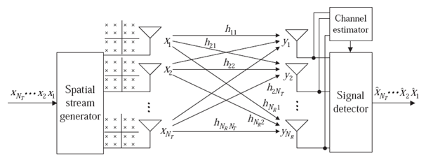 | Figure 1. SM-MIMO systems |
 th entry
  for the channel gain between the
  transmitting antenna and the
  receiving antenna,
  , and
, and  . The coefficients of
  describe all possible paths that data streams from different transmitting antennas may experience [7-9].The spatially-multiplexed user data and the corresponding received signals are represented by
 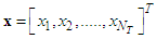 and
and 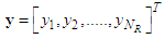 respectively, where
  and
and  denote the transmitted signal from the
  transmitting antenna and the received signal at the
  receiving antenna, respectively. Let
  denotes the white Gaussian noise with a variance of
  at the
  receiving antenna, and
  denotes the th column vector of the channel matrix
  . Now, the
  MIMO system is represented as
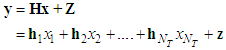 | (1) |
 [7-9,18].In [10] and [11], it was demonstrated that an impulsive noise model is a reasonably realistic description for many communications channels, including indoor and metropolitan wireless environments. Impulsive noise is characterized by heavy-tailed distributions and can be described by a number of statistical models. In order to evaluate the efficiency of examined algorithms, it was evaluated by using computer simulation according to the probability of demodulation error per 1 bit (BER) versus SNR, at different noise distributions. In terms of the realistic noise distributions, was used the generalized Gaussian distribution (GG) probability density function as shown in equation (2).
 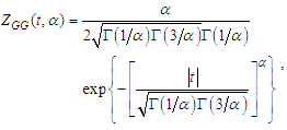 | (2) |
 (where
  is the gamma function), Distribution (2) is a priori unknown for all investigated detectors. GG-PDF in (2) has finite Fisher information and variance equal to 1 for all
  . For
. For  , GG distribution coincides with the Gaussian distribution and, while for
  the distribution coincides with the two-sided Laplace distribution. For
  , this distribution has heavier tails compared with the Gaussian distribution [8,9,18]. Fig. 2 shows a variety of densities at different values of
  .
. 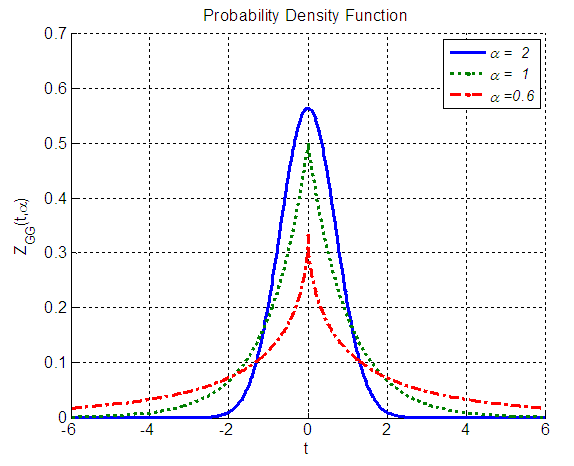 | Figure 2. Variety of noise distributions obtained by GG-PDF, at  and 0.6 and 0.6 |
3. Suboptimum Detectors
- A. Zero-Forcing DetectorIn MIMO, the task of the linear detector is to provide an estimate for each of the multiple transmitted symbols by performing only linear operations to the measured samples at the receive antennas. The primary advantage of the zero-forcing (ZF) detector is that it provides estimates for each transmitted symbol which contain no interference from the other transmitted symbols. It is also known as the decorrelator detector [12]. ZF detector used to nullify the interference by the following weight matrix:
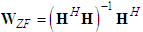 | (3) |
 is the Hermitian transpose operation. In other words, it inverts the effect of channel as
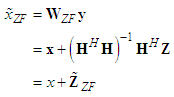 | (4) |
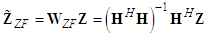 . Note that the error performance is directly connected to the power of
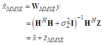
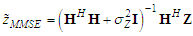
  [7-9,18].B. Minimum Mean Square Error DetectorWireless communication systems with the minimum errors at higher data rates can be obtained using SM-MIMO. With the assistance of SM-MIMO; the suboptimal MMSE detector is considered as a practical solution that can provide lower complexity and support higher data rates. MMSE detector strengthens the energy of the desired signal, and at the same time, it nullifies the unwanted interference by using its receive degrees of freedom such that the signal-to-interference-plus-noise ratio (SINR) is maximized. By using a MMSE linear detector, the wireless communication system transmission capacity was shown to be scaled linearly with the number of antennas at the receive end [3,13-15]. Also, the post-detection signal-to-interference plus noise ratio (SINR) can be maximized by using the MMSE criteria. The used MMSE weight matrix is given as
 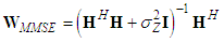 | (5) |
 is required. Note that the
  row vector
  of the weight matrix in (5) is given by solving the following optimization equation:
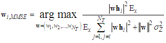 | (6) |
 | (7) |
 [7-9,18].C. Ordered Successive Interference Cancelation Detection Technique Generally, the linear detection techniques provide bad performance in comparison with nonlinear detection techniques. However, linear detection techniques require a low hardware complexity in the course of implementation. The performance of these linear detection techniques can be improved without increasing the hardware complexity by an ordered successive interference cancellation technique.
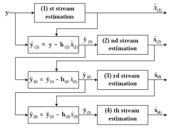 | Figure 3. OSIC detection approach for 4 spatial streams |
4. Proposed Robust Fair-based SM-MIMO Detector
- There are continuing efforts in order to develop detection techniques that achieving a near-optimal or optimal performance with less complexity. The proposed detector based on the use of Fair M-Estimator. M-estimators are one popular robust technique which corresponds to the maximum likelihood type estimate [17].Fair detector calculates the difference between the received signal vector and the product of all possible transmitted signal vectors with the given channel
 , calculates Fair function value at each difference, and hence determines the minimum Fair function value. Fair detector determines the estimate of the transmitted signal vector
  as
as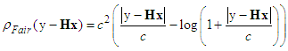 | (8) |
 | (9) |
 is a symmetric, positive-definite function with a unique minimum at zero. The value c is a tuning parameter that's used for trading-off high effectiveness with robustness. It was found that the tuning parameter c has 95% efficiency at 1.3998 [18,19]. The c=1.3998 tuning parameter was used in my simulation.
5. Simulation Results
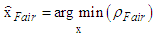
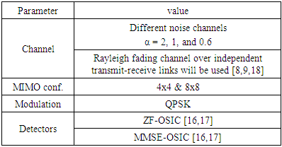
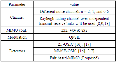
- The simulation results will be partitioned into three subsections A, B, and C as follow:A. Effect of Gaussian / non-Gaussian noises on the performance of examined detectorsSimulation parameters used in this part are shown in Table 1,
|
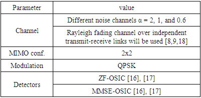
 | Figure 4. BER versus SNR performance, for ZF-OSIC, and MMSE-OSIC detectors, at α = 2, and 2X2 SM-MIMO system |
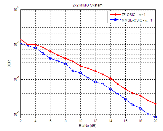 | Figure 5. BER versus SNR performance, for ZF-OSIC, and MMSE-OSIC detectors at α = 1, and 2X2 SM-MIMO system |
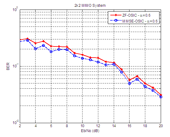 | Figure 6. BER versus SNR performance, for ZF-OSIC, and MMSE-OSIC detectors, at α = 0.6, and 2X2 SM-MIMO system |
|
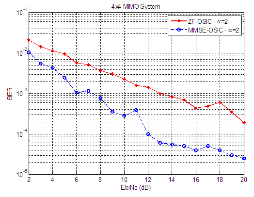 | Figure 7. BER versus SNR performance, for ZF-OSIC, and MMSE-OSIC detectors, at α = 2, and 4X4 SM-MIMO system |
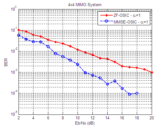 | Figure 8. BER versus SNR performance, for ZF-OSIC, and MMSE-OSIC detectors, at α = 1, and 4X4 SM-MIMO system |
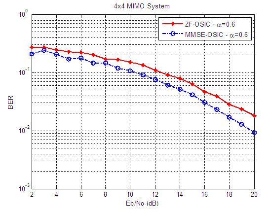 | Figure 9. BER versus SNR performance, for ZF-OSIC, and MMSE-OSIC detectors, at α = 0.6, and 4X4 SM-MIMO system |
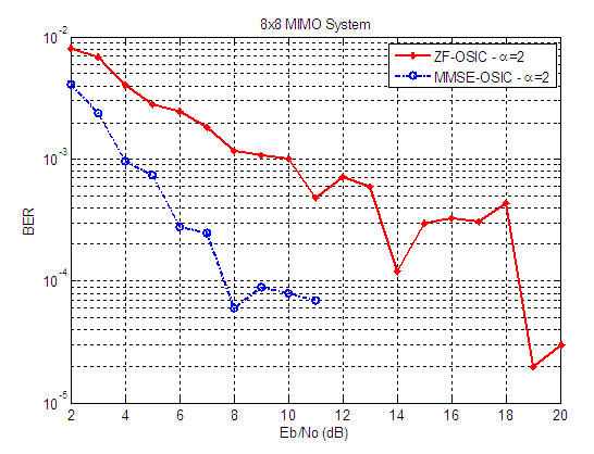 | Figure 10. BER versus SNR performance, for ZF-OSIC, and MMSE-OSIC detectors, at α = 2, and 8X8 SM-MIMO system |
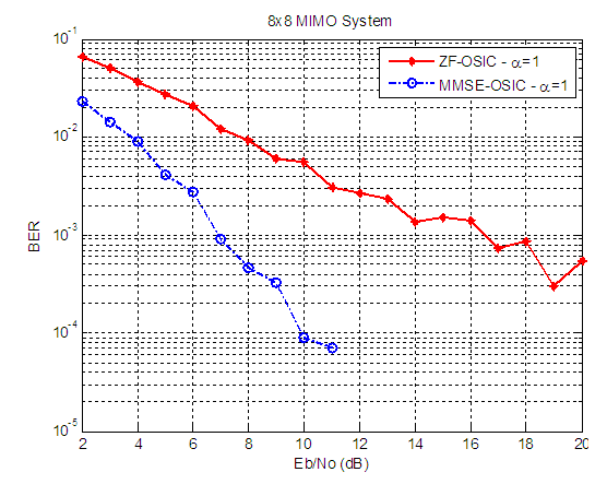 | Figure 11. BER versus SNR performance, for ZF-OSIC, and MMSE-OSIC detectors, at α = 1, and 8X8 SM-MIMO system |
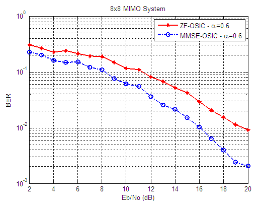 | Figure 12. BER versus SNR performance, for ZF-OSIC, and MMSE-OSIC detectors, at α = 0.6, and 8X8 SM-MIMO system |
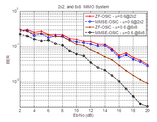 | Figure 13. BER versus SNR performance, for ZF-OSIC, and MMSE-OSIC detectors, at α = 0.6, and 2X2, and 8X8 SM-MIMO system |
|
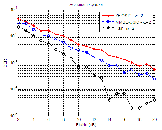 | Figure 14. BER versus SNR performance, for ZF-OSIC, MMSE-OSIC, and Fair detectors, at α = 2, and 2X2 MIMO system |
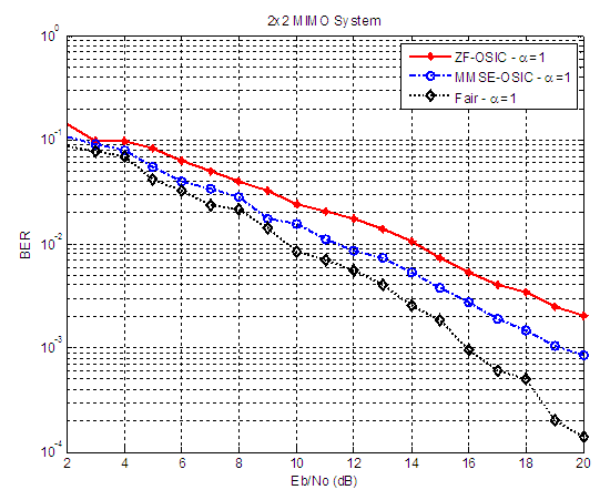 | Figure 15. BER versus SNR performance, for ZF-OSIC, MMSE-OSIC, and Fair detectors, at α = 1, and 2X2 MIMO system |
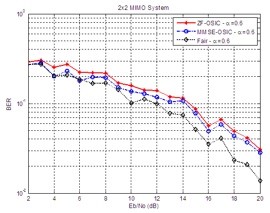 | Figure 16. BER versus SNR performance, for ZF-OSIC, MMSE-OSIC, and Fair detectors, at α = 0.6, and 2X2 MIMO system |
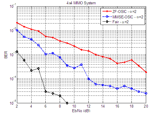 | Figure 17. BER versus SNR performance, for ZF-OSIC, MMSE-OSIC, and Fair detectors, at α = 2, and 4X4 MIMO system |
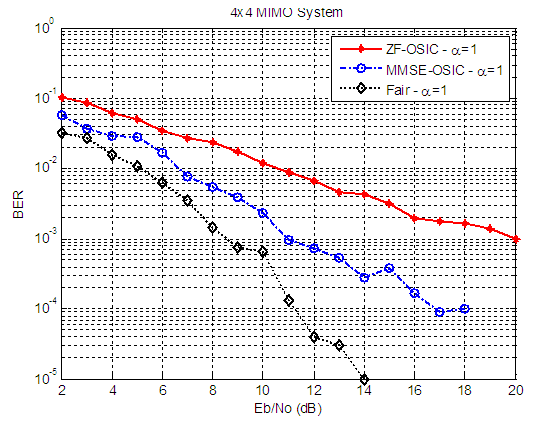 | Figure 18. BER versus SNR performance, for ZF-OSIC, MMSE-OSIC, and Fair detectors, at α = 1, and 4X4 MIMO system |
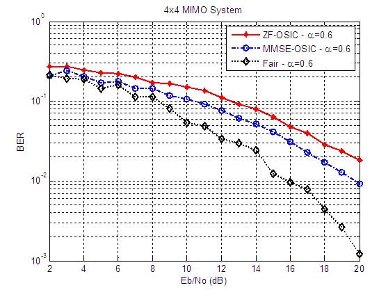 | Figure 19. BER versus SNR performance, for ZF-OSIC, MMSE-OSIC, and Fair detectors, at α = 0.6, and 4X4 MIMO system |
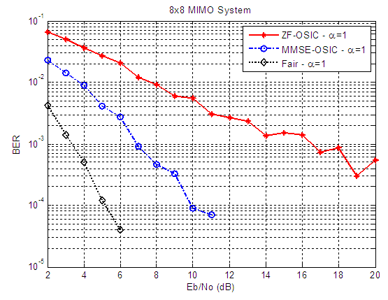 | Figure 20. BER versus SNR performance, for ZF-OSIC, MMSE-OSIC, and Fair detectors at α = 1, and 8X8 MIMO system |
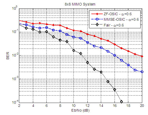 | Figure 21. BER versus SNR performance, for ZF-OSIC, MMSE-OSIC, and Fair detectors, at α = 0.6, and 8X8 MIMO system |
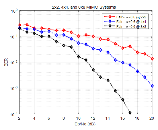 | Figure 22. BER versus SNR performance, for ZF-OSIC, MMSE-OSIC, and Fair detectors, at α = 0.6, and 2X2, 4x4 and 8X8 SM-MIMO system |
6. Conclusions
- The Fair-based SM-MIMO detector is proposed in this paper. The proposed detector outperforms the conventional linear MIMO detectors, including the ZF-OSIC and MMSE-OSIC detectors, at noise distributions. The proposed detector achieves a noticeable performance improvement where it successfully nullifies the Gaussian noise effect (at α = 2), and achieves BER=0, for the full range of SNR values, at 8x8 MIMO configuration. The proposed detector designed for LTE and LTE-advanced wireless communication systems.