1. Introduction

Smart cities initiatives are expected to have a large impact on the efficiency, safety, and sustainability of urban areas. Smart Cities involve augmenting city elements with Information and Communications Technologies. Buildings are a major source of energy consumption with around 40% of primary energy consumption across the globe. In addition, elements of smart city are concerned with increasing safety, comfort and productivity of city residents. In this paper we focus on smart buildings.

Building information modelling is an established technology in construction of engineered buildings. It builds digital representation and visualization of physical and functional entities of a building through capturing the characteristics, attributes and real-time status of building entities throughout the lifecycle of the building (pre- construction, during construction, and post-construction). Data collection is typically done through a set of sensors deployed across the building. In fact, proactive management of large buildings requires continuous and real-time performance monitoring. Building management agencies are under increasing pressure to adopt more proactive approaches to minimize impacts of failures. There is also a significant need to monitor many physical parameters in such buildings including: temperature, humidity, light intensity, sound intensity, rainfall intensity on the roof and others. Installing wired sensors in large structures is very difficult, costs a lot, and does not provide a flexible way for changing places of deployed sensors if needed.

Real-time management can be used for resource management: e.g. saving power by turning on/off lights, ventilators and air-conditions as needed. It can be also used in crowd management: giving a precise indication of occupied and empty spaces using camera sensors, providing direction signs to empty spaces in case of crowd, providing indication signs to evacuation routes in case of emergencies, and supporting statistical studies of crowd flow. It can be also used in maintenance management: providing a fire detection system, determining defects in the buildings’ structure to provide early maintenance, monitoring sound intensity all over the building and hence providing accurate control of the sound systems, and saving large amount of maintenance charges by allowing easy deployment and replacement.

Over the past two decades, numerous technologies and methods have been developed and deployed for such real-time monitoring. However, the installation and maintenance costs as well as the inherent limitations (e.g., power consumption, telemetry) of existing technologies constitute a major impediment towards implementing continuous real-time monitoring in a cost-effective manner. The efficiency and economic viability of current practices not only have limited the deployment of these technologies, but many infrastructure management agencies still do not have an effective or systematic strategy for infrastructure monitoring.

In recent years, advances in miniaturization; low-power circuit design; simple, low power, reasonably efficient wireless communication equipment; and improved small-scale energy supplies have combined with reduced manufacturing costs to make a new technological vision possible, namely Wireless Sensor Network (WSN) [1, 2]. A WSN consists of a group “motes” or “sensor nodes”. A mote or a sensor node is an autonomous, compact device, a sensor unit that also has the capability of processing and communicating wirelessly. The big strength of motes is that they can form networks and co-operate according to various models and architectures.

The aim of this paper is to implement a theoretical platform for a random WSN for monitoring applications in an irregular shape large building. We used Al-Masjid al-Haram “The Sacred Mosque” situated in Makkah al-Mukarramah “Mecca” as an example. The building is one of largest mosques in the world, if not the largest at all. It covers an area of about 356,800 square meters and can accommodate more than one million worshippers at a time. There is a significant need to monitor many physical parameters in the building, especially as it attracts a huge number of visitors mainly five times per day (for praying) and moreover during Hajj and Ramadan, when the number of visitors considerably increases. To the best of our knowledge there have been no studies for implementing WSNs in the holy mosque. Such a study is a vital issue, especially when considering the large area of the mosque and its importance.

The rest of the paper is organized as follow: section 2 introduces large scale WSNs with an overview on routing protocols used in that type of large networks. Section 3 gives an overview of the WSN simulator Cooja and the simulation model. Finally, section 4 presents the simulation results.

2. Large Scale WSNs

Large scale WSNs are formed by deploying large number of sensors in a large geographical area. The main WSN design objective is to achieve desirable coverage and accuracy while maintaining quality of service (QoS), cost, reliability, and scalability at acceptable levels. The network has a multiple hierarchical layout and employs a multi-hop wireless protocol to exchange messages and transmit data to base stations. Different software modules are developed to run at each level of the network hierarchy. A sensor node is typically powered by batteries. Sensors are designed to have sufficient intelligence to gather and disseminate data. Sensors can share information amongst the sensors themselves and cooperate in processing gathered data. This enables the network as a whole of monitoring a larger geographical area through large-scale distributed processing and communication of data performed by many sensors. A tutorial paper is introduced in [4], which is designed for both researchers and practitioners to provide a useful references and covers fundamental research for large WSN. The authors studied the theoretical foundations of such large-scale sensor networks. There are many fundamental organizational and operational issues related to large sensor networks that should be addressed: connectivity, sensor density, capacity, energy efficiency, and delay.

Although WSN can be used for a large number of applications, a number of general requirements characteristics are shared among most these applications. These characteristics include cost-effectiveness; longer service life, scalability, resiliency to faults, and privacy and security. Firstly, cost-effectiveness has always been one of the key design issues. Secondly, WSN should be able to operate as long as possible without recharging the batteries. Scalability involves ability to increase the size of coverage area in a manner that does not adversely affect WSN performance. Robustness involves ability of sensors and WSN to tolerate faults or errors in operations. This requires sensor nodes and WSN to have autonomous capabilities such as self-test, self-configuring and self-healing. The design of WSN must also incorporate security mechanisms in order to prevent unauthorized access and attacks. These requirements raise several major issues underlying WSN design and deployment and require a fundamental understanding of techniques for connecting and managing WSN nodes. This report provides a state-of-the-art review of WSN architectures, communication protocols, and data aggregation algorithms.

A major issue of concern is the connectivity of WSN, which is particularly important in sensor networks, where achieving a common application objective may require communication among all the nodes [3, 4]. The sensor density is an important factor in WSN in general and is of more significance in large area WSN, as it has large impact on connectivity, cost of the network, and data availability. Any proposed algorithm for WSN has to well compromise between these factors when determining the density of sensors, [5] has discussed the sensor density for partial connectivity in large area WSNs and it proved the existence of a critical sensor density around which the probability that at least a certain fraction of sensors are connected in the network increases sharply. In [6], sensor node saves the energy in node density field to increase the lifetime of WSN. Node density is uniformly distributed in hexagonal cluster to prevent the draining of battery and thus increases the lifetime of sensor network.

The capacity of large WSN has been discussed in [4, 7]. [4] explored how nodes can cooperate with each other in a large scale WSN and what are these networks capable of, more specifically the architecture of information transfer within the WSN. In [7], an upper and constructive lower bound for the data gathering capacity has been derived. The reliability of large WSN based on energy efficiency and network lifetime has been introduced in [3, 8], concentrating on improving the lifetime of the network based on energy efficient routing.

Finally, delay has been considered in some few papers. [9] presented a comprehensive delay performance measurement and analysis in a large-scale WSN through building a lightweight delay measurement system and present a robust method to calculate the per-packet delay. [10] introduced a monitor and rescue system integrating stationary and mobile wireless sensors. It concentrates on satisfying certain reaction delay requirement while minimizing the total cost and energy consumption.

A number of sensor networks protocol have been proposed for large WSN. In [11] an energy efficient routing protocol with multiple sinks has been proposed, which has been extended after that by the same authors in [12] for multiple mobile sinks. A scalable random routing protocol is proposed in [13], where scalability plays the key factor in the design of the protocol. Scalability is a challenging problem in WSNs that did not get enough attention of the researchers till now. A design for a mobile large scale WSN has been presented in [14], where a multi-radio and heterogeneity inspired architecture design scheme for mobile enabled wireless sensor network has been proposed. [15] provide a review for the communication protocols and algorithms in MAC layer and network layer, and examine the standard components in the sensor network architecture. Based on the survey, the authors recommended multi-hop and cluster based sensor network communication architecture for their proposed application.

3. Simulator and Simulation Model

A large variety of network simulators are available for simulating WSNs. Some of these varieties are network simulator platforms that have been specifically designed to model and simulate WSNs. Cooja [16], which is a part of Contiki [17] is an example for such a platform. Contiki is an open source operating system for the Internet of Things, connecting tiny low-cost, low-power, memory-constrained wireless systems. Contiki supports the recently standardized IETF protocols for low-power networking, including the 6lowpan adaptation layer, the RPL IPv6 multi-hop routing protocol, and the CoAP RESTful application-layer protocol.

The Contiki system includes the network simulator Cooja. A simulated Contiki Mote in Cooja is an actual compiled and executing Contiki system; the system is controlled and analyzed by Cooja. Cooja is a flexible Java-based simulator designed for simulating networks of sensors, where each node can be of a different type, differing not only in on-board software, but also in the simulated hardware. Cooja is flexible in that many parts of the simulator can be easily replaced or extended with additional functionality. Example parts that can be extended include the simulated radio medium, simulated node hardware, and plug-ins for simulated input/output. A simulated node in Cooja has three basic properties: its data memory, the node type, and its hardware peripherals. The node type may be shared between several nodes and determines properties common to all these nodes. For example, nodes of the same type run the same program code on the same simulated hardware peripherals, and also nodes of the same type are initialized with the same data memory. Cooja was originally developed for Cygwin/Windows and Linux platform, but has later been ported to MacOS.

The area used for simulation is the second floor of the building. There are few obstacles on the second floor, but they were neglected in our model. Figure 1 shows the map of the second floor (roof), which is used for the simulation. The simulation model consists of one stationary base station located in one corner of the irregular shape building. The number of wireless motes varies from 10 to 50 motes. All the nodes are homogenous, stationary and randomly distributed on the area. The nodes used in the simulation model are Tmote Sky nodes.

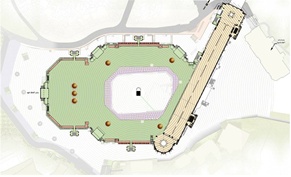Figure 1. Second floor or roof of Al-Masjid Al-Haram

The radio model used is the unit disk graph medium (UDGM) distance loss, where nodes communicate and interfere in fixed-radius circles. UDGM distance loss is an extension of first radio propagation model. In this model interferences are considered and packets are transmitted/ received with success ratio transmission/receive probability. The transmission rate in our model is fixed for all nodes and is equal to 1Mbps. The simulation parameters are number of nodes, transmission range, average transmission power and average number of hops.

A simple routing mechanism was used in the simulation, as the main purpose of the paper is to find out how will the number of nodes and transmission range affect the energy consumption and delay in the specified area of simulation. We used Cooja multihop module, which provides hooks for forwarding packets in a multi-hop fashion. The routing forwards every incoming packet to a random neighbor. List of neighbors is explored through neighbor’s discovery procedure and maintained using announcement mechanism. Also at least one route from each node to the base station is maintained through a route discovery procedure. Figure 2 shows the established connections for 20 nodes distributed randomly in the simulation area with transmission range of 60m.

Figure 2. Connections of 20 nodes randomly distributed

A node is disconnected from the network in two cases: the first when it consumes all its power, and the second when no route to the base station is available. When a packet arrives to a node, it picks a random neighbor to send the packet to. The packet is forwarded by the next node in the network until it reaches its final destination (or is discarded in transit due to a transmission error or a collision).

4. Simulation Results

We ran a large group of simulations for implementing a wireless sensor network in the mosque. The simulation runs were implemented having 10, 20, 30, 40 and 50 nodes. Moreover, in each group of the simulation the transmission range varied from 20m to 100m with a step of 20m. This makes a total of 25 simulation runs. Figure 3 through Figure 7 show the remaining average amount of power dedicated for transmission (abbreviated transmit power) versus the average on-time of sensor motes (abbreviated on-time).

Figure 3 shows the transmitted power vs. on-time for 10 nodes randomly distributed. For the transmission range 20m, the network is not connected, this is because of the small number of nodes (10 nodes) and the small transmission range, and hence the nodes are out of range of each other. We have indicated non-connected networks by a zero-line in the graphs. It is clear – from the figure – that the power consumed is decreased by increasing the transmission range. This happens because the number of hops needed to reach the destination is decreased by increasing the transmission range, and hence the average power dissipated is decreased, but this is valid up to an optimum value, which is here the transmission range 80m. Increasing the transmission range more than 80m in case of 10 nodes, will not save power, as the number of hops will not be decreased. The figure shows that for transmission range of 100m, the power consumed is increased by about 20%.

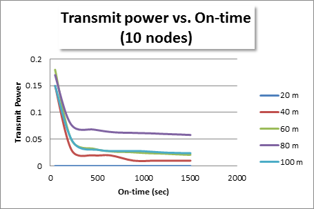Figure 3. (Transmitted power vs. On-time for 10 nodes randomly distributed)

On the other hand, the lifetime of the network can be also deduced from the figure. The lifetime can be determined when the power level comes to a saturation value, at that level a certain number of nodes are of out power, so that the network is not connected anymore. That is why the level becomes constant after a while as there is almost no more power consumption, because there are no more transmissions. The 100m range has a better power consumption distribution among the nodes, and hence it has larger lifetime.

Figure 4 shows transmitted power vs. on-time for 20 nodes distributed randomly. The 40m range has both better power performance and greater lifetime, which makes it the best choice for this network. In Figure 5, the best lifetime is almost the same for 60m, 80m, and 100m. However, it is better to choose the 60m choice for lower power consumption and to decrease the collision probability. Figure 6 considered 40 nodes distribution. The best performance in that case is the 60m range, as before for both parameters considered, the lifetime and the average power consumed.

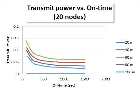Figure 4. (Transmitted power vs. On-time for 20 nodes randomly distributed)

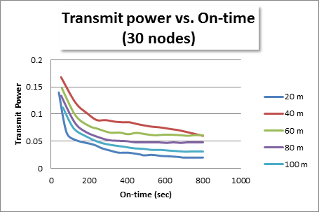Figure 5. (Transmitted power vs. On-time for 30 nodes randomly distributed)

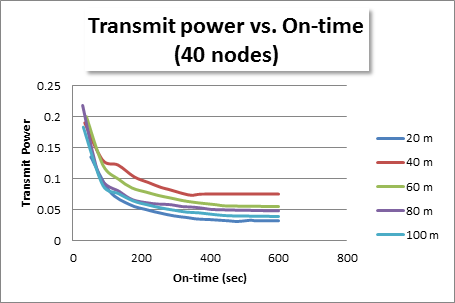Figure 6. (Transmitted power vs. On-time for 40 nodes randomly distributed)

In the case of having 50 nodes randomly distributed (Figure 7); the best performance appears when using the 20m range. This is clear as the increase of the number of nodes allow the nodes to send over a small range and still reach the sink (base station). The 20m range gives also the best lifetime and almost the best power consumption. The 100m has a low performance because of the collisions that will appear when using relatively a large number of nodes and a high transmission range.

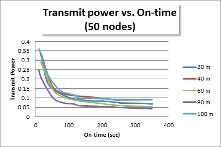Figure 7. (Transmitted power vs. On-time for 50 nodes randomly distributed)

From the previous results, it is clear that by increasing the number of nodes and hence the node density, the performance is better for the lower transmission ranges. Using the results, one can choose the optimum transmission range according to the number of nodes needed, or vice versa, i.e. the best number of nodes according to a certain transmission range.

At the end of this group of simulation results comes the average number of hops vs. number of nodes and transmission range. The average number of hops also represents the average delay. According to the transmission rate, packet size and number of hops, the delay can be calculated easily as follows:

Delay = (packet size / transmission rate) * number of hops

From Figure 8, it is clear in general that the number of hops decreases by increasing the transmission range. This is logic as each mote sending with higher transmission is considered logically more close to the sink, as it can reach the sink by less number of hops. Still there are some exceptions in the graph. For 10 nodes, 40m and 60m ranges have lower number of hops than the 80m; this can be explained by considering the previous figures; this happens because the network is disconnected early as the nodes away from the sink are almost not connected to the sink because of the limited range, only some nodes near the sink are connected. In the mentioned cases, the average number of hops is low, but still this is not a good choice as the network is not fully connected.

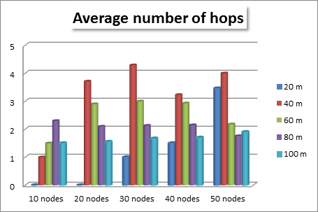Figure 8. (Average number of hops vs. number of nodes and transmission range for random distribution)

For 20 nodes, it is straight forward and average number of hops is decreasing with increasing the transmission range, here also for the 20m transmission range, the network is not connected at all.

The same for 30 and 40 nodes with one exception, namely the 20m range as shown clearly on the figure, which is also because the network is not fully connected because of the low transmission range in case of 20m transmission range, which is the same as explained for the 10 nodes case.

In the case of 50 nodes, the number of hops for 80m and 100m are so close; this is because there is almost no difference between both transmission ranges for such a large number of nodes (50 nodes). The number of hops for 100m is higher only because the traffic is random, so any of them can be slightly higher than the other according to the traffic of each case.

5. Conclusions and Future Work

The presented research simulates different scenarios for wireless sensor networks randomly distributed in an irregular shape large building. The area used in the simulation model, is the “Sacred Mosque”. This objective is innovative, as to the best of our knowledge no such research has been proposed before to implement WSNs in the holy mosque. The research presents the relation between average number of hops versus the total number of nodes in the network for different transmission ranges, and also shows the average transmit power dissipated over the time for different number of nodes and different transmission ranges. In addition, the network lifetime can be determined from the power consumption graphs. Using the results, one can choose the optimum transmission range according to the number of nodes needed, or vice versa, i.e. the best number of nodes according to a certain transmission range.

The simulation parameters are number of nodes, transmission range, average transmission power and average number of hops. Simulation figures show the relation between average transmission power and on-time for different number of nodes and different transmission range scenarios. From the figures one can deduce the best transmission range or best number of nodes for a specific scenario. The simulation results clearly show that the power consumed is decreased by increasing the transmission range. This happens because the number of hops needed to reach the destination is decreased by increasing the transmission range, and hence the average power dissipated is decreased. This is valid up to an optimum value, which is shown for each transmission range. Increasing the transmission range more than the optimum value, will not save power, as the number of hops will not be decreased and hence consuming more power. The average number of hops vs. number of nodes and transmission range is also represented in the simulation figures, in general that the number of hops decreases by increasing the transmission range.

Future work will include simulation of nodes having uniform distribution over the mosque and a comparison between uniform and random distributions. Also an implementation that presents the obstacles in the mosque will be considered.

ACKNOWLEDGMENTS

This research has been supported by the Center of Research Excellence in Hajj and Omrah (HajjCoRE), Umm Al-Qura University, Makkah, Saudi Arabia. Under Project number P1126, titled “Intelligent Wireless Sensing for Monitoring Applications at the two Holy Mosques”.

We would like to thank Abrar Al-Hindi and Maria Al-Sheikh for helping in the simulation results.