Visvasuresh Victor Govindaswamy1, Gergely Záruba2, G. Balasekaran3
1College of Art and Sciences, Concordia University Chicago, Illinois, 60639, United States
2College of Computer Science and Engineering, The University of Texas at Arlington, Texas, 76019, United States
3Human Bioenergetics Laboratory, Nanyang Technology University, Singapore, 639798, Singapore
Correspondence to: Visvasuresh Victor Govindaswamy, College of Art and Sciences, Concordia University Chicago, Illinois, 60639, United States.
| Email: |  |
Copyright © 2014 Scientific & Academic Publishing. All Rights Reserved.
Abstract
In this paper, we extend the work done on stochastic modelling of Random Early Detection with Explicit Congestion Control (RED-ECN) gateways to present a mathematical model for Random Early Detection with Receiver Window Modification (RED-RWM) gateways, a novel TCP congestion control approach, which could be used with any of the present Active Queue Management (AQM) schemes, such as Random Early Detection (RED), Adaptive Random Early Detection (ARED), and BLUE queues to further reduce congestion at the ingress and gateway routers. We also provide an asymptotic and steady-state analysis for the model and show that 1) the average TCP dynamics for a large number of flows using a RED-RWM queue is closely related to that of a single flow utilizing the same TCP congestion control mechanism and that 2) the sessions become asymptotically independent as number of flows using the queue becomes large, suggesting that the RED-RWM queue alleviates the synchronization problem among the flows. We use a Monte Carlo simulation method to compare outcomes of our mathematical model with outcomes of NS2 simulation experiments. In earlier published works, we had shown that RWM schemes complementing RED, Blue and ARED queues easily outperform RED, Blue and ARED queues functioning with and without ECN. Hence, by using the mathematical model, one can predict the outcome of the scheme before implementing it.
Keywords:
TCP, Active Queue Management (AQM), Buffer Management, Random Early Detection (RED), Congestion Control, Congestion Avoidance, Random Early Detection with Receiver Window Modification (RED-RWM), Explicit Congestion Control (ECN), Receiver Window Modification (RWM)
Cite this paper: Visvasuresh Victor Govindaswamy, Gergely Záruba, G. Balasekaran, Mathematical Modeling of the RED-RWM Active Queue Management Scheme, Journal of Wireless Networking and Communications, Vol. 4 No. 2, 2014, pp. 49-65. doi: 10.5923/j.jwnc.20140402.03.
1. Introduction
TCP is the connection oriented transport layer protocol of the Internet. One of the services TCP provides is the cutting back on the transmission rate of flows whenever a congestion is encountered on the way of the packet flow. Such congestion at routers may be caused by too many sources trying to send an excessive amount of data with a rate too high for the network to handle. Originally at routers new incoming packets were dropped whenever the queue of the router was already full. To provide better feedback to the TCP sending processes (to enable them to detect and react to congestions earlier) various queue management schemes have been proposed; they can be divided into two categories: i) passive queue management algorithms, where the queue of the routers needs to fill up before corrective action is taken; and ii) active queue management (AQM) [1], where preventive action is taken before the queue is saturated. Modeling and analysis of TCP connections with queues has been an active research area. In [2], a Markov chain based model is analyzed for N TCP connections using either Tail-Drop or RED gateways [3], where the state space is the vector of window size of all of the N connections, the queue size is a function of the sum of the size of congestion windows and state transition probabilities are dependent on packet loss probability at the router buffer, and the SS and CA phases of TCP. Many of the past work assume that the packet loss probability is constant but it is in fact dependent on the buffer size and packet discarding discipline at the router and the window size of the transmission. In [4], the authors use a previously developed nonlinear dynamic model of TCP to analyze and design RED by relating its parameters such as the low-pass filter break point and loss probability profile to the network parameters. Finally, Tinnakornsrisuphap et al. [5] have modeled a RED queue with TCP connections that explicitly incorporate complete packet level operations in TCP, probabilistic packet marking mechanism in RED, heterogeneous round trip times (RTTs) of TCP flows and session-layer dynamics, i.e., connection arrivals and departures. Their model avoids the state space explosion of as well, however assuming that the RED queue does not drop packets. In this paper, we present a mathematical model for the Receiver Window Modification (RWM) scheme introduced in [6], [7], [8] that can be used to complement the RED scheme at the ingress and gateway routers. In [7], we showed that RWM schemes complementing RED, Blue and ARED queues easily outperform RED, Blue and ARED queues functioning with and without ECN. Our model in this paper extends the modeling work done in [5] in detail to the RWM extension, henceforth to the RED-RWM, relaxing the assumption that the buffer size infinite. Here, upon selection of packets, the RED-RWM queue, instead of marking them, sets the receiver window field to one maximum segment size (MSS) in the ACK packets that are going towards the sender from the receiver. The main idea of the RWM approach is to restrict the TCP transmission window with the flow control window instead of the congestion control window, thus controlling the transmission window with a finer granularity. Results from simulations show [7] that RWM extended queues out perform their counterparts (functioning with and without ECN) in terms of packet drops, packet delay, delay jitter and throughput.The rest of the paper is organized as follows: Section 2 covers the necessary background information and previous work. In Section 3, the RWM model is introduced; simulation details, results as well as analysis are covered in Section 4. The paper is concluded in Section 5.
2. Background Information
This section gives an overview of the various major topics involved in active queue management research. After a short general introduction, subsections 2.1 and 2.2 provide an overview of the RED AQM and the RWM scheme respectively.
2.1. Random Early Detection
The purpose of Random Early Detection (RED) [3] is to make the network more capable of accommodating bursty traffic rather than shaping bursty traffic to accommodate the needs of the network. It has two thresholds: Thmin and Thmax. If the average queue length is smaller than Thmin then the arriving segment is accepted. If the average queue length is between Thmin and Thmaz, then the segment is dropped with probability Pa. Pa is a linear function of the average queue length, possibly increasing to a pre-determined maximum value Pmax. However, if the calculated average queue length is larger than Thmax then incoming segments are dropped with probability one. This behavior results in a larger virtual queue size for short-term bursts compared to long-term bursts. The RED algorithm has also a glaring disadvantage when it comes to handling malicious flows [9]. Several schemes such as the many variants of the CHOKe [10] [11] algorithm such as the xCHOKe [12], RECHOKe [9] and RCUBE [13] algorithms have been proposed to remedy this disadvantage.In [5], Peerapol et al. have presented a RED model that deals with TCP transmission rate in terms of packet-level operations. Our RED-RWM model is an extension of this model, hence it has the following adopted features:1. Incorporates a more accurate Additive Increase / Multiplicative Decrease (AIMD) window mechanism of TCP. The AIMD algorithm controls the window size in response to the modified acknowledgement packet from the bottleneck RED-RWM gateway.2. Provides a more realistic session-level dynamics, i.e., arrivals and terminations of flows, and the variability of round-trip delays.3. Provides a realistic interaction between TCP and RED-RWM gateway.
2.2. Receiver-Window Modification (RWM)
AQM solutions, such as RED use packet drops at router queues to manipulate the TCP sender into decreasing its transmission rate. With ECN [14]-compliant RED queues, packets are not unnecessarily dropped but marked as if they were dropped. However, as a downside: i) ECN messages may get lost or dropped by downstream routers; and ii) TCP implementations at both the source and the destination have to be ECN-compliant (which presents a significant problem in today’s implementations). Currently there is no practical benefit in setting ECN bits in Internet packets; as this requires ECN capable routers (at least at bottleneck points), and servers and clients throughout a network. In [15], experiments were conducted using TBIT (the TCP Behavior Inference Tool) showing that in September 2000 only 21 out of 26447 (0.07%) sites positively responded with an appropriate SYN/ACK. In March 2002, only 7 out of 12364 sites (0.05%) responded positively. These tests included sites running nearly all types of operating systems.In [8], we had proposed in using flow control feedback to reduce congestion at ingress and gateway routers. Instead of setting ECN related bit in the chosen packets of RED queues, we proposed the use of receiver window modification (RWM). RWM sets the receiver window field to one maximum segment size (MSS) in the ACK packets that are going towards the sender from the receiver1. (Note that whenever the TCP header of an ACK packet is modified, the checksum in the TCP header needs to be adjusted for error control.) The advantages of RWM queues are that they work with the current implementation of TCP in end systems and do not require drastic changes to the existing network schemes. Hence, they overcome the disadvantages of the ECN queues since TCP/IP stacks will not require modifications to be “ECN-compliant”. Since, the feedback loop extends from the RWM queue on a router to the sender; the response of the algorithm is determined by the delay between the router and the sender rather than the RTT of the connection, which is true in the case for the queues using the ECN mechanism (assuming that there are other ACK packets “flowing” from the receiver to the sender). The delayed response of the sender to an ECN is further compounded if the congestion worsens at the other routers lying between the router and the receiver. The response time will also be heavily dependent on the types of queue implementations in these routers. The queues using the RWM mechanism enjoy the advantage of faster response times to the impending congestion since the notification of congestion arrives at the source quicker when compared to those using ECN mechanism. In [7], we showed that RWM schemes complementing RED, Blue and ARED queues easily outperform RED, Blue and ARED queues functioning with and without ECN.
3. RED-RWM Model
This section presents the model for the RED-RWM gateway with N TCP connections competing for bandwidth. We expand on the model developed for the ECN/RED gateway in [5].We will discretize time T with a uniform duration ΔT and make use of timeslots represented by [t*ΔT, (t+1)* ΔT) where t is an integer starting at 0 (thus we will be talking about timeslot t or time t*ΔT). The round-trip times (RTTs) of TCP connections are approximated as integer multiples of the length of timeslots (ΔT). We define a logical indicator function we denote: 1 [L] which evaluates to 1 if L is true and to 0 if L is false. We also define the following variables:1) fm(N)(t): R+ → [0,1]: the feedback (segment acknowledgement modifying) probability function in the RED-RWM gateway when there are x number of packets in the queue being used by N number of sources. Hence, the probability of acknowledgements being modified or segments being dropped by the RED-RWM gateway is fm(N)(t). (fm(N)(t) should scale with N.)2) fd(N)(t): R+ → [0,1]: the segment dropping probability function in the RED-RWM gateway when there are x number of packets in the queue being used by N number of sources. The same rules apply to fd(N)(t) as to fm(N)(t). 3) Q(N)(t): the queue size at time ΔT*t with N number of TCP connections. During timeslot t, this size will increase or decrease if the number of incoming packets at the queue is greater or less (respectively) than the number of outgoing packets.4) Ai(N)(t): the number TCP segments received by the RED-RWM gateway from TCP connection i (i є {1,…,N}) within timeslot t; thus, the total number incoming segments at the RED-RWM queue is: | (3.1) |
Ai(N)(t) can be modeled by an integer-valued random variable that encodes the transmission window size (in packets) at time ΔT*t; we assume that Ai(N)(t) є {0,…,Wmax}, where Wmax represents the receiver advertised window size of the connection (the transmission window size of an idle connection is zero). 5) C(N)(t): the number of TCP segments served by the RED-RWM gateway during time slot t. 6) Since the queue is always non-negative, using the above variables, the queue dynamics can be represented by the following recursive function:  | (3.2) |
In addition, both A(N)(t) and C(N)(t) follow some stochastic recursions which depend on the current queue size thereby forming a stochastic feedback system. If we denote the average queue serving capacity per connection by C, then C(N)(t)=NC, thus Equation (3.1) becomes: | (3.3) |
7) Wi(N)(t): the transmission window size at connection i at the beginning of timeslot t. The transmission windows size is the minimum of cwnd and rwnd. We assume that each connection will transmit all TCP segments that it can during slot t. Note, that Ai(N)(t)≤Wi(N)(t). (More precisely if Φi(N)(t) is the number of pending TCP segments for connection i at time ΔT*t and connections have an unlimited amount of segments to transmit, then Ai(N)(t)=Wi(N)(t)- Φi(N)(t).)8) Xi(N)(t): the remaining workload (in packets) at the TCP sending process of connection i at the beginning of timeslot t; thus, Ai(N)(t) ≤ min(Wi(N)(t),Xi(N)(t)). (More precisely, Ai(N)(t)=min(Wi(N)(t)-Φi(N)(t),Xi(N)(t)) )9) Di(N)(t): the round trip time (RTT) at time t*ΔT as observed by the TCP sending process of connection i; Di(N)(t) will be given in integer multiples of ΔT. We model Di(N)(t) as a random variable of possible outcomes: {2,…,Dmax}.10) We will assume that any congestion-control action occurs at the end of a round-trip. We also simplify the segment transmissions to the queue by assuming that all segments allowed within an RTT are transmitted in the same slot to the queue. Let βi(N)(t) represent the number of timeslots (at timeslot t) since the last time connection i has transmitted a segment to the queue; then:
 With these assumptions our formula for Ai(N)(t) will evolve to:
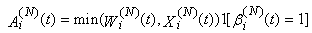 where the indicator function
  is to ensure that the connection transmits only once per RTT. (Note, that the above assumptions eliminate the need for variable Φi(N)(t).) Now our formula for the queue evolution can be rewritten as:
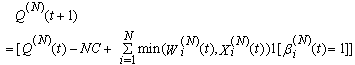 | (3.4) |
11) Let us introduce function Gi,t(a,b) evaluating to a if the last transmission action of connection i at time t*ΔT was within the then applying roundtrip time, and evaluating to b otherwise. G will be a useful tool to change variables only after a RTT has passed. | (3.5) |
12) Let the modifying and dropping probability functions [16] be given by: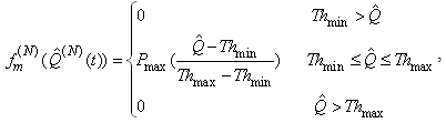
 where Pmax is the maximum marking probability, Thmin is the minimum threshold, Thmax is the maximum threshold. 13) Since the RED-RWM scheme complements the RED queue, it uses the same queue averaging filter as the RED queue (known as Exponentially Weighted Moving Average -EWMA) to evaluate the average queue size based on the instantaneous queue size with a past-weighting parameter α (0< α ≤ 1). Let
  represent average queue at time t*ΔT, then:
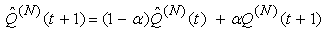 | (3.6) |
14) Let zi,j(N)(t+1) represent random indicator variables for dropped packets, where j є {1, ...,Ai(N)(t)}; zi(N)(t+1) is zero if the jth packet of connection i is dropped in timeslot t (and 1 otherwise). Thus:  where Li,j(t)s are I..I.D. (in all their dimensions) uniform random variables taking values from [0, 1]. Hence, the indicator function of the event that no packet of connection i is dropped in timeslot t can be written as:
 If zi(N)(t+1)= 0, then at least one packet from connection i in timeslot t has been dropped by the RED-RWM gateway. This information may only be used one RTT later to halve the value of the congestion window size, thus we need to propagate a zero value to the end of the roundtrip time. We will use variable Zi(N)(t) for such propagation. Zi(N)(t) thus evolves according to:
 Now we can define variable
  to reflect that there was a drop during the previous RTT.
  evolves according to
  | (3.7) |
15) Similarly, let the modification of acknowledgement packets by the RED-RWM gateway be represented by an indicator random variable mi,j(N)(t+1) where j є {1, ...,Ai(N)(t)}; mi,j(N)(t+1) is zero if the jth packet of connection i causes the acknowledgement packet to be modified by the RED-RWM gateway to one MSS in timeslot t:  where Vi,j(t)s are I.I.D. (in all their dimensions) uniform random variables taking values from [0, 1]. Hence, the indicator function of the event that no packet of connection i is RWM-modified in timeslot t can be written as
 If mi(N)(t+1)= 0, then at least one packet from connection i in timeslot t has been RWM-modified by the RED-RWM gateway. This information may only be used one RTT later to modify the transmission to 1 MSS, thus we need to propagate a zero value to the end of the roundtrip time. We will use variable Mi(N)(t) for such propagation. Mi(N)(t) thus evolves according to:
 Now we can define variable
  to reflect that there was a modification during the previous RTT.
  evolves according to:
  | (3.8) |
16) Connection i, after receiving the modified acknowledgement from the RED-RWM gateway, will transmit only one MSS for one RTT. After the RTT the source will transmit the minimum of the previous congestion window before modification and the new advertised receiver window (unless it receives more modified acknowledgements from the RED-RWM gateway). Thus, we need to save the transmission window’s size before the RWM modification has happened using variable Ωi(N)(t). Ωi(N)(t) evolves according to: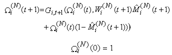 | (3.9) |
17) We also need an indicator variable at each roundtrip’s end time, showing whether there has been a marking two roundtrips ago while there has been none in the roundtrip that was just finished. 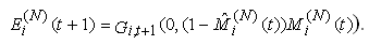 | (3.10) |
18) Each connection may be in one of two basic modes i.e., either in an active or an idle mode. At the beginning of timeslot t if a session has no packet to transmit then it is in the idle mode. An idle connection may become active by the beginning of the next timeslot with probability par independently of previous events. Hence the duration of an idle period is geometrically distributed with parameter par (and a mean of 1/par). We can use this to capture the dynamics of connection arrivals, where the interarrival times are exponentially distributed (as the geometric distribution is the discrete equivalent to the exponential distribution), we let i) Ui(t) (i є {1,…,N}) represent a collection of I.I.D. uniform random variables on [0, 1] and ii) 1 [Ui(t+1) ≤ par] represent an indicator function for an idle connection i for the event of the arrival of a new packet in timeslot t+1.19) Let Fi(t) represent the total number of TCP segments (the session size) connection i will have to transmit if it becomes active at the beginning of timeslot t; Fi(t) can be modeled as a collection of I.I.D. non-negative integer-valued random variables with some general probability mass function (usually a geometric or a discretized exponential pmf).Recall, that we used Xi(N)(t) to denote the remaining workload (expressed in TCP segments) of connection i at the beginning of timeslot t; thus: 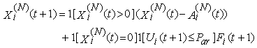 | (3.11) |
20) RTT will not change for a connection during the same RTT, thus we can formulate it using the Gi,t(a,b) function. At the beginning of time slot t+1 (if t+1 is the timeslot for connection i to send its data) the expected roundtrip time is determined by the proportion of how many segments are in the queue at time ΔT*(t+1) plus how many are expected during slot t+1 (which is A(N)(t+1)) and the rate with which the queue is served: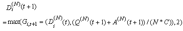 | (3.12) |
Note, that this can lead to synchronization if we assume that all connections arrive at the same time. This synchronization will be removed by the random marking and dropping as t grows. The above formulation also requires Di(N)(t) to be at least two as we expect the acknowledgments to come back in a different time slot than what was used to send their segments.21) The evolution of the window mechanism for connection i can now be described through recursion. The congestion-control mechanism of TCP operates either in the slow start (SS) or the congestion avoidance (CA) phase. A new connection starts in SS in order to probe the available bandwidth of the network (the queue in our case). While in SS, the congestion window size is doubled every round-trip time until the receiver window field of one or more acknowledgement packets are modified by the RED-RWM gateway to one MSS or one or more packets are dropped by the RED-RWM gateway. Note that the transmission window size is limited by the receiver advertised window size Wmax. Thus, if the connection is in SS then the transmission window of connection i evolves according to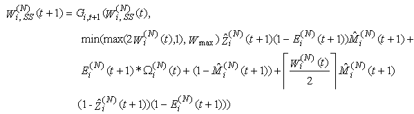 | (3.13) |
22) In CA, the congestion window size in the next timeslot (t+1) is incremented if no modified acknowledgement packet was received in timeslot t, while if one or more segments are modified in timeslot t the congestion window in the next timeslot is set to one segment. The congestion window size in CA is then given by: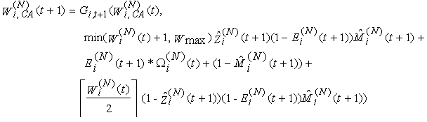 | (3.14) |
23) Let the Si(N)(t) random indicator variable denote the state of TCP connections (Si(N)(t) is zero if connection i is in CA and one if it is in SS). Therefore, combining Equations 314 and 315, the complete recursion of the congestion window size can be written as: The last indicator function is used to reset the congestion window size to zero when connection i runs out of data and returns to its idle state. 24) Finally, the evolution of Si(N)(t) can be described as:
  | (3.15) |
where connection i will be in the SS state during timeslot t if there is either i) no packet left to transmit (so the connection resets) at the beginning of the timeslot or ii) the connection was active and in the SS state then a packet drop or marking leads to the CA state. Equation 315 assumes that a new TCP connection, in the SS state, is set up one timeslot after the previous connection is torn down upon finishing its workload, and the new TCP connection becomes active when a new file/object arrives, initiating a three-way handshake. Moreover, it implies that the state is updated in the next timeslot following a transmission despite the window size being updated one RTT after transmission using the appropriate SS/CA state as in the correct operation of TCP.
3.1. Asymptotic Analysis
Here, we present a theorem for the asymptotic analysis for the RED-RWM queue when the number of connections using the queue is large. Firstly, we present the initial conditions and then the theorem.(Initial condition 1) For i = 1, . . .,N, the initial conditions of random variables in the model are: 
 and
and We denote the vector of state variables for connection i in timeslot t by
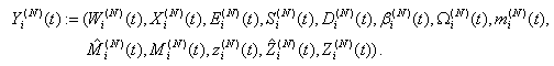 | (3.16) |
(Initial condition 2) All TCP connections are responsive to congestion control and the number of connections N is greater than the value of Thmin.Theorem 1. i. Assume that both Initial Conditions (1 and 2) are valid and  where
where  denotes weak convergence or convergence in distribution with large N, then the sequences
 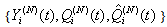 and
and  with t= 0, 1, 2, 3…. are time-homogeneous Markov chains, i.e. their future states are dependent on the present state and not on past states.ii. Given the recurrence of the RWM model as
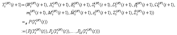 with the state space Y given by
 Then it holds by analysis that
  are given by
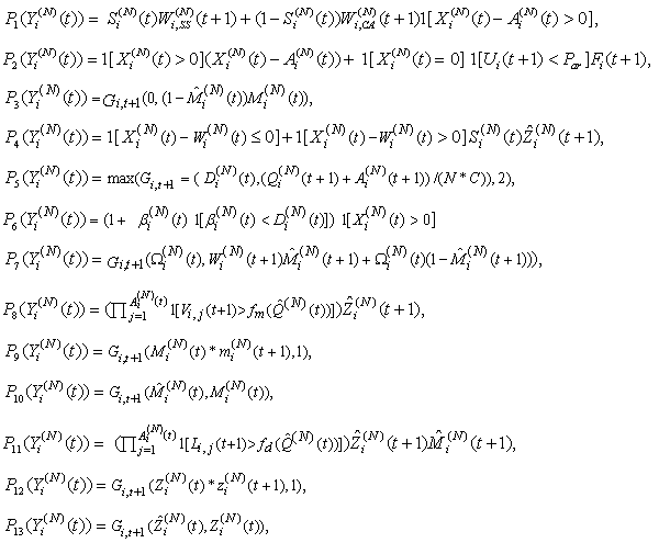 where
where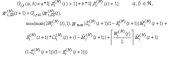 and
and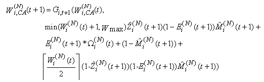 for i.i.d. [0, 1]-uniform rvs { Li,j(t + 1), Ui (t + 1), Vi,j (t + 1); t = 0, 1, . . .}.iii. For any bounded function
  , we have
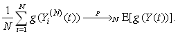 where
where  and
and denotes convergence in probability when N tends to infinity, with the state space Y given by
  and
and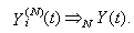 where
where  denotes weak convergence or convergence in distribution with large N.Here, we are implying that the average TCP dynamics for a large number of flows using a RED-RWM queue is closely related to that of a single flow utilizing the same TCP congestion control mechanism.iv. For any integer i = 1, 2, . . . , the random vector
  becomes asymptotically independent as N becomes large, with
 for any yi є Y, i = 1, . . . , I.Here, we are implying that as sessions become asymptotically independent as N becomes large, suggesting that the RED-RWM queue alleviates the synchronization problem among the flows.v. For large N, we have
 and
and Resulting in
 vi. For any bounded mapping
  there exists a bounded and continuous mapping
  such that
 | (R1) |
This assumption states that given the events leading up to the beginning of timeslot [t, t + 1), the expected behavior of session i leading to the beginning of timeslot [t + 1, t + 2) can also be determined using the expected knowledge of the conditional receiver window modifying probability,  , the conditional dropping probability
  and
and  . Hence, (Assumption 3) implies that
 | (R2) |
This leads to (from iii) | (R3) |
implying that for large N, given the events leading up to the beginning of timeslot [t, t + 1), the expected behavior of session i leading to the beginning of timeslot [t + 1, t + 2) can also be determined using the expected value of the conditional receiver window modifying probability,  , the conditional dropping probability
  and
and  .
.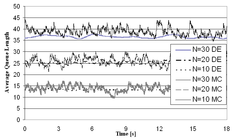 | Figure 1. Average queue length at a RED-RWM queue |
The proof of Theorem 1 is shown in Appendix 1. Limiting CasesNext, consider the resulting model from Theorem 1 in the regime when C is either very large or very small.C is large: the modifying probability per flow converges to zero for all t. Therefore, each incoming flow will always operate in the SS mode with each connection doubling its window sizes every round-trip. C is very small: the average queue size increases with the modifying probability. The rate of modifying acknowledgements increases as the modifying probability approaches 1. As a result, an increasing number of TCP connections will receive modified acknowledgements and will approximately transmit a single packet. If the dropping probability is 1, packets will be dropped.
3.2. Steady-State Analysis
Here, we present a theorem for the steady-state analysis for the RED-RWM queue when the number of connections using the queue is large.(Initial condition 3) The sequence  with t = 0, 1, 2, 3…. admits a steady state such that
 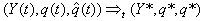 where
where  is a constant and
  is a y-valued rv.Theorem 2. Assume that both Initial conditions (1, 2 and 3) and Theorem 1 are valid. Let us use the notation:
  to denote a weak convergence in N to a steady state. Then:
 See Proof is shown in Appendix 2 of this paper.
4. Simulation Results and Analysis
We have created an NS2 [17] model of the RED-RWM scheme. (The NS2 TCP-Reno model has to be corrected as it does not follow a common linux-type TCP implementation with the interaction of restricted contention and flow control windows). We used a simple barbell topology with a single congested link and varied the number of connections N from 10 to 30. All connections were modeled as “File Transfer Protocol (FTP)” flows, i.e., as constant and inexhaustible source of information. We used the following RED parameters.• Queue weight given to current queue size sample =0.002 • Minimum threshold of average queue size (Thmin) = N-1• Maximum threshold of average queue size (Thmax ) = 3N• Max probability of dropping a packet = 1/linterm, where linterm = 3The average queue sizes were observed and depicted in Figure 1. It can be observed, that RWM helps RED in keeping the average queue within the bounds, closer to the Thmin threshold.To verify our formulation we have also created a custom Monte Carlo simulation implementing the analytic equations. We have performed simulation with parameters similar to those of the discrete event simulation. The average queue sizes were observed with both methods and are depicted in Figure 1; curves with a DE suffix are results of the discrete event simulations (NS2) while curves with an MC suffice show the Monte Carlo results (analytic). (Note that the time frame of these two simulations is not identical but plotting them on the same figure, i.e., their variation may not be on the same time scale). We can observe a good match, validating our mathematical model (note, that more extensive simulations have been performed with changes in other parameters and those results underline this conclusion as well).
5. Conclusions
In this paper, we have presented a mathematical model for the RED-RWM queue by extending the work done previously for RED-ECN queues. We have verified our model by comparing Monte Carlo simulations of our model to discrete event simulations of an NS2 model. We “theoretized” that the RWM modified RED queue will weakly converge to a steady state and that as the number of clients (TCP connections) grows, the queue size will weakly converge to the number of clients, assuming that the minimum marking threshold (Thmin) is less than the number of clients. We are currently working on research to • Implement RWM in Linux based packet routers and by using various flavors of TCP with multi-bottleneck topologies.• Control congestion with an extended-RWM (ERWM) scheme at the edge routers to ensure that at the borders of the network that each flow's packets do not enter the network faster than they are able to leave it. The aim here is to push any complexity in controlling congestion toward the edges of the network by not modifying the core routers and the end systems.
Appendix 1
Proof of Theorem 1:The sequence  is a stochastic process with a finite number of states in which the probability of occurrence of a future state is conditional only upon current state; past states does not matter. Considering an arbitrary bounded mapping
  and writing
  as function of
  through a case analysis, it can be seen that the above argument is correct. The states that
  can transition from [t,t+1) are as follows:
 where
where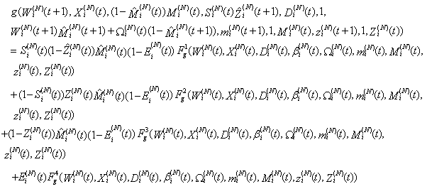 The mappings
  and
and  are associated with g and defined by:
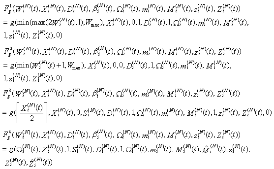 We introduce the following terminology to facilitate the proof of the theorem: For each t = 0, 1,…., the statements [A:t], [B:t], [C:t] and [D:t] below refer to the following convergence statements:[A:t] There exist some non-random constants
  and
and  such that
 [B:t] For some {0, 1, …, Wmax} g-valued rv
  , non-negative integer-valued rvs
  and {0,1}-valued rvs
  it holds that
 [C:t] For any integer i = 1, 2, . . . , the random vector
  becomes asymptotically independent as N becomes large, with
 where
where  is given as in [B:t].[D:t] For any bounded function
  , the convergence
 holds with
  in [B:t].[E:t] For any bounded mapping
  there exists a bounded and continuous mapping
 such that
 | (R1) |
This assumption states that given the events leading up to the beginning of timeslot [t, t + 1), the expected behavior of session i leading to the beginning of timeslot [t + 1, t + 2) can also be determined using the expected knowledge of the conditional receiver window modifying probability,  , the conditional dropping probability
  and
and  at [t, t + 1). Hence, it also implies that
 | (R2) |
This leads to | (R3) |
implying that for large N, given the events leading up to the beginning of timeslot [t, t + 1), the expected behavior of session i leading to the beginning of timeslot [t + 1, t + 2) can also be determined using the expected value of the conditional receiver window modifying probability,  , the conditional dropping probability
  and
and  .Lemma 1: If [A:t], [B:t] and [C:t] hold for some t = 0, 1, …, then [D:t] holds.Proof: From [B:t] and Proposition 4.7, Pg. 140 [55], if
  and
and  is a continuous function, then
 . It immediately follows that
 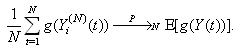 Hence, [D:t] holds.Lemma 2: If [A:t] and [B:t] hold for some t = 0, 1, …, then [E:t] holds.The random vector
  for a session i in timeslot [t, t + 1) takes values
 and
and  in a discrete space Y. Hence, the rv
  can be determined as a function of
  , i.e.,
  , for some bounded continuous function
  Letting
  , we define
 to be the conditional probability that, given
  connection i will receive receiver window modification acknowledgements from the RED-RWM gateway during the period [t, t + 1). Under the enforced independence assumptions, it is clear that
 Letting
  , we also define
 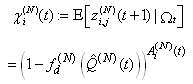 to be the conditional probability that, given
  connection i will experience packet drops by the RED-RWM gateway during the period [t, t + 1). Under the enforced independence assumptions, it is clear that
 Finally, it follows from (R3)
 | (R4) |
 | (17) |
where the mapping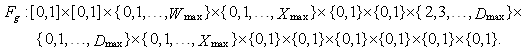 By using 316 to substitute
  in 17, we get
 | (18) |
Taking expectation on both sides, we get Since
Since  is continuous on
  and using Proposition 4.7, Pg. 140 [55],
 Hence
Hence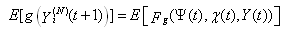 | (19) |
Hence [E:t] holds.Lemma 3: If [A:t], [B:t] and [C:t] hold for some t = 0, 1, …, then [C:t+1] holds.Proof: From [C:t], we have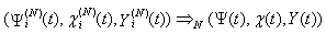 Since
Since  is independent of
  . We can see that
  by using 18.By Bounded Convergence Theorem,
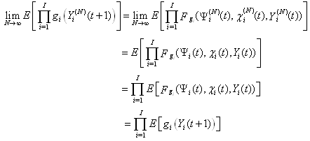 | (20) |
From 20 and using the Bounded Convergence Theorem, we can see that 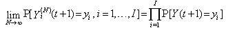 Lemma 4: If [A:t] and [D:t] hold for some t = 0, 1, …, then [A:t+1] holds.Proof: From [D:t], we can conclude that
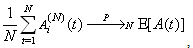 and from [A:t],
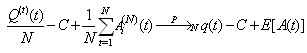 Since
Since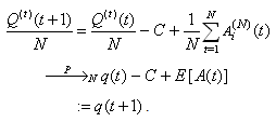 Since from [A:t],
  and
and  we get
 Since from above,
  we get
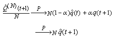 Lemma 5: If [A:t] and [B:t] hold for some t = 0, 1, …, then [B:t+1] holds with Y(t+1) related in distribution to Y(t)Proof: From 19, we have
  Since g is a bounded mapping function, it follows that
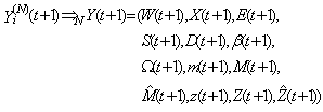
Appendix 2
Proof of Theorem 2:Assume the following:i. Average queue size ( ) is currently N-1, where thmin = N-1. (This ensures that the next packet will trigger the RWM scheme.)ii. The RWM queue modifies the receiver window in the acknowledgements to 1 MSS for every packet arrival after the thmin threshold.Using, from [3],
  we get
 | (6.1) |
Simplifying this further, as N is varied from 1 to 500 and setting  = 0.002, we get
 Hence, in Equation (61),
  | (6.2) |
If, for example, the first packet, which enters after  has reached the thmin, is from flow i, then the RWM queue will modify flow i’s acknowledgement to 1 MSS. This implies that in the next RTT, flow i will transmit only a single packet. Since there are N numbers of connections, at the steady state, all N connections will transmit a single packet. Since the number of packets in the queue will be approximately N and hence, greater than the thmin threshold, the RWM scheme will be triggered continuously until congestion eases.Next, we relax the assumption ii to figure out the number of packets beyond the thmin that can be queued without triggering the RWM scheme that will lead to
  to just exceed N+1. Let M represent the number of packets. Table 1 shows the results of the increase in the instantaneous queue length to render such a situation.Since the Equations 38, 3-13 and 3-14 (and thus the RWM scheme) is triggered often whenever the average queue is between thmin and thmin thresholds, well before these M values have been reached, Equation 62 holds true.
| Table 1. Results of the increase in the instantaneous queue length for the different number of connections |
| | Number of Connections | M | | 10 | 90 | | 50 | 195 | | 100 | 257 | | 200 | 328 |
|
|
Note
1. Some researchers claim that routers in general should not look at layer-4 headers as their function is limited to layer-3. Yet, enabling them to do so can provide significant benefits (see e.g., NAT).
References
| [1] | M. Kwon, and S. Fahmy, A comparison of load-based and queue-based active queue management algorithms, Proceedings of the International Society for Optical Engineering, pp. 35-46, vol. 4866, July/August, 2002. |
| [2] | G. Hasegawa and M. Murata, Analysis of dynamic behaviors of many TCP connections sharing Tail–Drop/RED routers, Proceedings of IEEE GLOBECOM, November 2001. |
| [3] | S. Floyd and V. Jacobson, Random early detection gateways for congestion avoidance, IEEE/ACM Transactions on Networking, pp. 397-413, vol. 1, no. 4, August, 1993. |
| [4] | C. Hollot, V. Misra, D. Towsley, and W. Gong, A control theoretic analysis of RED, Proceedings of IEEE INFOCOM, 2001. |
| [5] | P. Tinnakornsrisuphap and R. La, Limiting Model of ECN/RED under a Large Number of Heterogeneous TCP Flows, Technical Report, Institute for Systems Research, University of Maryland, 2003; Proceedings of IEEE Conference on Decision and Control (CDC) 2003, Maui, Hawaii, December 2003. |
| [6] | V. V. Govindaswamy, G. Zaruba and G. Balasekaran, “Analyzing the Receiver Window Modification Scheme of TCP Queues” in Proceedings of the 2006 INFOCOM, 25th IEEE International Conference on Computer Communications. pp.1 – 6, 2006. |
| [7] | V. V. Govindaswamy, G Záruba, G. Balasekaran, Easing Congestion in Computer Networks using the Receiver-Window Modification (RWM) Scheme, International Journal of Networks and Communications (Vol.2, No.5, September 2012). |
| [8] | V. V. Govindaswamy, G. Zaruba and G. Balasekaran, “Receiver-Window Modified Random Early Detection (RED-RWM) Active Queue Management Scheme: Modeling and Analysis” in Proceedings of the 2006 IEEE International Conference on Communications, vol.1, pp.158–163, 2006. |
| [9] | V. V. Govindaswamy, G Záruba, G. Balasekaran, “RECHOKe: A Scheme for Detection, Control and Punishment of Malicious Flows in IP Networks”, IEEE International Conference on Communications (ICC 2007), Glasgow, Scotland, UK, 24-28 June 2007. |
| [10] | R. Pan, B. Prabhakar, and K. Psounis, “CHOKe: a stateless active queue management scheme for approximating fair bandwidth allocation”, Proceedings of IEEE INFOCOM, volume 2, pp. 942–951, Tel Aviv, Israel, March 2000. |
| [11] | V. V. Govindaswamy, G Záruba, G. Balasekaran, “Analyzing the Accuracy of CHOKe Hits and CHOKe-RED Drops”, Electrical and Computer Engineering, 2008. CCECE 2008. Canadian Conference on, Glasgow, Scotland, UK, 24-28 June 2007. |
| [12] | C. Parminder, C. Shobhit, G. Anurag, J. Ajita, K. Abhishek, S. Huzur, S. Rajeev, xCHOKe: Malicious Source Control for Congestion Avoidance at Internet Gateways. Proceedings of IEEE International Conference on Network Protocols (ICNP-02), Paris, Nov 2002. |
| [13] | Govindaswamy, V. V.; Zaruba, G.; Balasekaran, G., Receiver Window Modified Random Early Detection Queues with RECHOKe, Electrical and Computer Engineering 2009 (IEEE CCECE'09), Conference: Symposium on Communications and Networking, On page(s): 142-147, 3-6 May 2009. |
| [14] | S. Floyd, TCP and Explicit Congestion Notification, ACM Computer Communication Review, pp. 10-23, vol. 24, October, 1994. |
| [15] | TBIT, the TCP Behavior Inference Tool.http://www.icir.org/tbit/ecn-tbit.html. |
| [16] | Probability Theory and Mathematical Statistics for Engineers. Paolo L. Gatti, London: New York: Spon Press, 2005. |
| [17] | NS2 simulator http://www.isi.edu/nsnam/ns/ |
 Abstract
 Reference
 Full-Text PDF
 Full-text HTML