C. Mikeka1, M. Thodi1, J. S. P. Mlatho1, J. Pinifolo2, D. Kondwani2, L. Momba2, M. Zennaro3, A. Moret3
1Physics Department, Chancellor College, University of Malawi
2Malawi Communications Regulatory Authority (MACRA)
3T/ICT4D Marconi Wireless Lab, Abdus Salam, International Center for Theoretical Physics (ICTP)
Correspondence to: C. Mikeka, Physics Department, Chancellor College, University of Malawi.
| Email: |  |
Copyright © 2014 Scientific & Academic Publishing. All Rights Reserved.
Abstract
Performance status of the Malawi TVWS pilot as of December 2013 is presented. Basic performance metrics like throughput, latency, SNR have been analyzed using known path loss empirical models like Hata, Asset and Friis. Additionally, this paper presents new data mining tools developed using Python and Perl which were deployed at each TVWS station’s ALIX board running on Voyage Linux to abstract useful data for computation of network latency and throughput. Typically, for the longest tested link at 7.5 km, an average SNR = 24.7 dB, data-rate of 420 kbps and latency of 118 ms were observed using the collected data. Empirically, Hata and Asset resolved an average path loss value equal to 155 dB which was 51 dB higher than the ideal Friis Free Space Path Loss (FSPL) at UHF CH31 (554 MHz), BS antenna height of 23 m, receiver antenna height of 2m, and farthest station distance of 7.5 km. These results prove a 2.6 times superior propagation performance of the TVWS network over the commercial fixed broadband wireless network (assuming 2 Mbps backhaul, and all other parameters controlled). These measurements were done in dry season. Results for rainy season will be studied from December 2013 to June 2014.
Keywords:
Latency, Python, SNR, Throughput, TVWS
Cite this paper: C. Mikeka, M. Thodi, J. S. P. Mlatho, J. Pinifolo, D. Kondwani, L. Momba, M. Zennaro, A. Moret, Malawi Television White Spaces (TVWS) Pilot Network Performance Analysis, Journal of Wireless Networking and Communications, Vol. 4 No. 1, 2014, pp. 26-32. doi: 10.5923/j.jwnc.20140401.04.
1. Introduction
While the expectations from using TVWS for wireless broadband service are high, the commercial and technical viability of TVWS operations is still largely unknown [1]. Several researchers have studied the use of TV white spaces for other applications [2-5]. In 2011, [3] carried out a technical feasibility on the use of TV White Spaces for broadband access in different sectors namely; rural and urban with the potential for traffic offload from congested mobile broadband networks, ‘Smart city’ applications and location-based services. The primary aim of the study in [3] was to assist Ofcom in developing the regulatory framework which was to facilitate the use of TV white spaces and help improve spectrum efficiency and provide universal broadband access. One of the key findings of the study was that TV white spaces spectrum can be used for a range of applications, from improving rural broadband connections to machine-to-machine (M2M) applications. Similar studies have also been carried out in USA and Singapore. Most of the studies on TV white spaces have either focused on the availability of the TV white spaces, advances in TV white space radios or the development of TV white spaces regulatory framework and white space device specifications [3-8]. Very few studies, to the knowledge of the authors, have focused on the performance of a deployed TV white space network. Of the few TV white space network deployments in Africa, the network performance analysis has not been published. Thus, this paper presents a performance of the TV white spaces network under harsh African environment for example intermittent power and constrained Internet bandwidth resource. This work also presents low cost and innovative tools for monitoring and analysing TV white space networks.An evaluation of the performance of well-defined secondary systems in realistic scenarios will eventually help to gauge the market prospects for TVWS-driven technologies and potentially guide subsequent regulatory rule-making. In Malawi, the partnership team between the regulator (referred to as the Authority in the TVWS regulations) and the University of Malawi, Chancellor College have in the mid of December, 2013 developed the TVWS rules and regulations, investor side business model and a performance analysis of the network since deployment. The goals for the Malawi TVWS Pilot are similar to that of the Cambridge Trial [9] which intends to help industry understand the capability of TV white spaces to serve a wide range of applications, through key factors such as the coverage and performance that can be achieved. The rest of this paper is organized as follows. Section II presents the network setup and the proposed method for the definition of the performance indicators or metrics and their analyses. Results are presented in Section III while Section IV discusses the results. Conclusions are drawn in Section V.Motivation for the TVWS Deployment in Rural MalawiA number of rural communities in Malawi have complained about the unavailability or poor broadband performance from the currently available commercial ISP services. Their experience is not unusual in Africa and other rural areas of the developing world. The key attraction of TV white spaces in this application is the enhanced coverage distances which lower frequencies enable (compared to the higher frequency bands traditionally used for wireless broadband access). The extended range translates into fewer base stations being required to cover a given area and, hence, lower CAPEX and OPEX costs. An additional advantage of subsidized license-scheme (ISM band-like) proposed in the December 2013 Malawi TVWS regulation draft, is that rural communities would have the capacity to provide their own wireless networks in the iconic fashion called citizen-science.In the Malawi pilot, measurements were made to establish the coverage and performance that could be achieved around pilot base station (BS) in the network setup as depicted in Section II. Measurements were taken with a spectrum analyzer at street level height of 2m connected to a TVWS Yagi antenna pointing to the BS, with checks on both received signal level (RSSI) and data throughput (uplink and downlink). The coverage achieved matched reasonably well with predictions made using Friis, Okumura-Hata, and Asset propagation modeling tools in a quasi-line of sight condition [6, 10] and script data mining tools using Python and Perl.The path loss estimations described in this paper will provide guidelines for researchers and practicing engineers in choosing appropriate path loss model(s) for coverage optimization and interference analysis for wireless devices operating in the TV band in our environment and also, to predict TV coverage and keep-out distances for potential secondary users operation in the TV white spaces [10].Another challenge for TVWS radio transceiver is the choice of the best digital hardware to meet the requirements. Features like flexibility, performance and power consumption are key factors for cognitive radios [11]. In the Malawi TVWS network the hardware can mitigate intensive interference by invoking adaptive modulation functionality in the base station communication subsystem. The manufacturer of our radio equipment is working on auto channeling for future products. To extend the coverage range further than the current 20km tested range, a study is in progress to use UHF band power amplifiers with fast switching capability to increase transmit power above the current 4W towards 10W using 50dB gain UHF amplifiers.The authors herein have previously published on the findings of a TVWS spectrum measurement initiative in Malawi and Zambia [12]. In [12] they introduced an open hardware device that geo-tags spectrum measurements and saves the results on a micro SD card. The device can also be used to record the use of spectrum over long periods of time. An assessment study on TV white spaces in Malawi using affordable tools was presented in [13]. In this paper, however, the scope is on the performance of the network since it is mandatory that appropriate performance indicators of cognitive radio systems (White Space Devices, WSDs) are identified [14].
2. Malawi TVWS Network Setup and Proposed Methods for Capturing Network Data
The Malawi TVWS network topology assumes a star configuration. It has a single base station and three client stations as shown in Table 1.| Table 1. Station identification in the online Operation and Management Center (OMC) |
| | Terminal | Description | Station Name | | CST00162 | ICTP CPE 162 | St. Mary’s Girls Sec School | | CST00163 | ICTP CPE 163 | Malawi Defense Force Air-wing | | CST00164 | ICTP CPE 164 | GPS (Seismology Dept.) | | CSB00490 | ICTP Base 490 | ZA TVWS Base Station (BS) |
|
|
2.1. Station Design and Description
Each station comprises client premise equipment (CPE) and a Yagi-Uda type of antenna mounted outdoors and powered by a UTP cable that terminates into an indoor Power-over-Ethernet (PoE) adapter. Additional station devices include a LAN switch and an ALIX board (functionality discussed in later sections). The TVWS base station is an indoor device, and has ultra-low power consumption compared with cellular base stations. It transmits using a huge monopole antenna (case of Carlson radios) mounted outdoors at a height based on rigorous computations or simulation per design coverage and link quality of the star topology.Internet supply in the Malawi TVWS pilot network is provisioned through a dedicated 2Mbps wireless backhaul as shown in Fig. 1. The actual network deployment terrain and coverage scope is shown is Fig. 2. | Figure 1. Malawi TVWS pilot network: Base station located at the GPS coordinates: -15.376415S, 35.318349E |
 | Figure 2. Malawi TVWS terrain coverage scope |
2.2. Low Cost Monitoring Platform
The network was deployed using Broadband Rural- Connect equipment from Carlson Wireless Technologies. The Carlson equipment comes with a cloud based Operation and Management Center (OMC) which provides a cloud level view of the devices that you register under a given name. This online tool is used for the initial configuration as well as management of the network. The OMC has graphical displays of SNR (uplink and downlink), application data throughput (uplink and downlink) as well as application packet throughput (uplink and downlink). The data presented in OMC has one major shortfall in that it cannot be saved or exported in any format for later viewing or analysis. Therefore the performance data in the OMC is only useful when one only wants to see the current performance and not the trends over a period of time beyond 24 hours. This prompted the authors to identify some low cost innovative tools of capturing and saving performance data using Python and Perl.To enable the real time collection of performance data, ALIX boards running Voyage Linux were fitted at each client station. i. Installation of Voyage Linux and Configuration of the Network Interfaces on ALIX boardsVoyage Linux was installed on the ALIX board using the procedure described in [15].After successful installation, Voyage Linux was mounted (with the compact flash (CF) card still connected to the Linux machine used for the installation) on /mnt/cf (the mounting point set in the installation configuration). Then, one network interface (eth0) was enabled and given an IP address (192.168.x.y/24). The configuration was saved; the CF card was un-mounted and slotted it into the ALIX board which was then booted.The interface eth0 connects to the client radio (the CPE) and another interface (eth1) was configured to be providing dynamic IP addresses in the range 192.168.0.5/ to /240 to computers on the client side using DHCP. The DHCP server used was dnsmasq whose configuration file is /etc/dnsmasq.conf. The interface itself was configured with a static IP address (192.168.0.1). ii. Python ScriptsGiven the limitations of the OMC, a need arose to have custom scripts that would capture and save network throughput data. For this purpose, Python programming language was chosen because it has numerous existing open source libraries and modules that can be used as-is as well as modified to suit different needs. The developed scripts were used to collect network and packet throughput data. The data was collected for each day on a one second interval. The collected data was then saved using comma separated values (CSV) files; chosen mainly for their portability. The files used the date stamp for the name for easy sorting and identification during analysis. Fig. 3 below shows a snippet of the data.The columns in each row contain the information; interface, bytes sent, bytes received, packets sent, packets received, bytes sent per second, bytes received per second, packets sent per second, packets received per second and time in that specific order. In addition to the scripts that capture throughput data, we also used some Python scripts to plot the data obtained into graphs. We mainly exploited the plotting functionalities of the matplotlib module for this purpose.iii. Perl Scripts The Python scripts that were developed did not capture network latency data. For this purpose, other scripts were developed in Perl programming language to capture and save network latency from the base station to all the clients’ sites. Again, the same Python language could have been used, but Perl was opted for due to the relative ease found by the researchers. | Figure 3. A snippet of the data stored in csv file |
3. Results
The important results in this paper are on the throughput, latency and path loss. Throughput and latency are computed averages from the measured data over one month at station premises. The path loss is computed using known empirical models with all equation variables replaced by the actual deployment parameters and conditions. Any assumptions made and limitations observed have been discussed in the subsequent sections.
3.1. Performance Graphs
The downstream throughput (blue line) and upstream throughput (black line) are shown in Fig. 4 below.  | Figure 4. Average downstream throughput at the farthest TVWS station, Airwing (7.5 km from BS) |
The average latency in milliseconds (ms) for 3rd December in an hour study is shown in Fig. 5 below. | Figure 5. One hour latency measurement at AirWing station |
Latency and overall throughput is dominated by two factors namely; the length of the route that the packets have to take between sender and receiver and the interaction between the TCP reliability and congestion control protocols. To confirm this point, a plot for latency at GPS station (closest station from TVWS BS) is shown in Fig. 6 below, where it is evident that the latency is lower than for the farthest station. The reduced latency however is not proportional to the scale factor of the station distance ratios because latency is a function of several factors. These include; propagation delay, serialization, data protocols, routing cum switching, and queuing cum buffing. Of the aforementioned factors, the determinant for the reduced latency between the shortest and farthest stations in this case is propagation delay. Propagation delay, in our case, is a function of how long it takes the information to travel at the speed of light in the wireless channel at 554 MHz from source to destination. These results are comparable to TENET study, the South African TVWS Trial [16].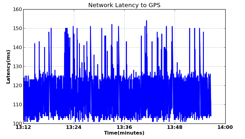 | Figure 6. One hour latency measurement at GPS Station (1.7 km from BS) |
3.2. Equations
In this subsection, path loss will be estimated based on Friis Free Space Path Loss (FSPL), Hata and Asset models. . Path loss estimation is the basis for the derivation or computation of the received power at a given station from the known base transceiver station. 1) Estimating Friis Path LossThe fundamental aim of a radio link is to deliver sufficient signal power to the receiver at the far end of the link to achieve some performance objective. For a data transmission system, this objective is usually specified as a minimum bit error rate (BER). In the receiver demodulator, the BER is a function of the signal to noise ratio (SNR) measured in decibels (dB).In designing a spectrally efficient wireless communication system like TVWS, it is important to understand the radio propagation channel. The characteristics of the radio channel will change mainly due to the operating frequency and the propagation environment. Typical examples may include line of sight (LoS) compared to non-line of sight (NLoS). In this work, all the stations are deployed in a quasi-NLoS environment. The major LoS obstructions are due to buildings, hills and trees which impose a slow fading condition over the channel. For shorter distances to the base station, it is still viable to employ Friis model given receiver antenna height of 2 meters above street level ground.The actual received power  at each TVWS station was calculated using (1) which has taken into account; system losses and antenna gain for the transmitter and the receiver.
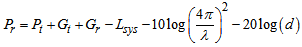 | (1) |
Where  = Receive power in dB
 = Transmit power in dB
  = Antenna gain for transmitter
 = Antenna gain for receiver
 =System losses
 = Distance
 Where
Where  = speed of light,
  The computed received power
  is shown in Table 2 below.
Table 2. The computed received power

 |
| |
|
The computed received power took into account the following path losses:  = 91.9 dB for GPS, 94.9 dB for St. Mary’s and 104.8 dB for AirWing. These results compared very closely to the actual spectrum measurements for GPS and St Mary’s (closest stations) at 554 MHz (given 20 MHz observation window) using a handheld spectrum analyzer terminated to the TVWS Yagi antenna (given same cabling losses). The measurement results for Malawi Defense Force AirWing were worse than the value presented in Table 2. A typical measurement was unsteady around -103 dBm on average at 2 m height and only improved to -93.8 dBm or better when the antenna height position was raised to 8 m above street level ground. These observations attracted the authors to estimate the path losses using other models like Okumura-Hata and Asset.Unlike Friis Free Space Path Loss (FSPL), Hata and Asset are realistic models because they take into account real environment factors such as reflection, scattering, diffraction, refraction and absorption of signals by many features such as vegetation, buildings and people hence ideal for modelling a network. Asset model closely resembles Hata model. Nevertheless, Asset model differs from Hata models because of the additional diffraction and clutter losses. The two formulae are presented in (2) and (3) below.2) Asset Propagation Model
 | (2) |
3) Hata Propagation Model | (3) |
Where, = Transmitting frequency (MHz)
 = Effective antenna height of base station (m)
 = Antenna height of the CPE station (m)
 = CPE height correction factor
 = Distance between CPE and base station (km)
 = Diffraction loss
 and
and  = Intercept and slope corresponding to a constant offset in dBm and a multiplying factor for the logarithm value of distance
 = CPE antenna height correction factor
 = Multiplying factor for
 = Effective antenna height gain
 = Multiplying factor for
 = Multiplying factor for diffraction loss
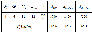
 = Clutter lossThe computed path loss comparison is shown in Fig. 7 where Hata compares closely to Asset as expected. However, Asset exhibits a 1.04% increment factor on the path loss compared to Hata which is due to the inclusion of the diffraction and clutter losses. Future work will include a careful study on the comparison of the measured received power to simulations based on these empirical models. In this work, the authors have simply confirmed the superiority of the Asset model to Okumura-Hata in path loss estimation. However, the authors think that the unity values assumed by the multiplying factor for the diffraction loss (K7) and the clutter loss are too ideal.
 | Figure 7. Computed path loss (a comparison between Friis Free Space, Hata and Asset Models) |
4. Discussion
The results presented in the preceding sections have demonstrated the superiority of Hata and Asset models over Friis FSPL in terms of the precision of the calculated path loss. At AirWing TVWS station, the measured SNR was equal to 24.7 dB implying a noise level of -118.5 dBm. There is however, a small correction on the effective receive-side antenna height during the computation of Hata and Asset path losses. The smallest antenna height of 2 m as deployed at St. Mary’s TVWS station was used to provide the worst case scenario for the computed path loss (deliberately done to simulate an NLoS environment). In reality the antenna height for GPS is 3 m while for AirWing is 8 m (to approximate LoS condition).In this paper, the downstream throughput could be defined by DTavg, then for AirWing, reading from Fig. 4 250≤DTavg≤420kbps. This data rate is 2.6 times better than the typical data rates (at 176kbps) provided by commercial operators in rural areas, given the same backhaul internet bandwidth of 2 Mbps. The commercial operators use 5.8 GHz ISM band Ubiquiti radios in Wi-Fi hotspot fashion.
5. Conclusions
In this paper, performance analysis of the TV white spaces in the UHF band in Malawi was performed. It is observed that unlike other fixed broadband services, TVWS services demonstrated 2.6 times better data rates given the same operating conditions.The longest tested operational range for the Malawi TVWS network is 18.56 km with the lowest SNR i.e. below 10 dB (Pirimiti station). However, the tested functional range at the moment is 7.5 km (AirWing) which measures an SNR of 24.7 dB, average latency of 118 ms and maximum throughput of 420 kbps given simultaneous usage of three client stations from a TVWS BS backhauled to a 2 Mbps internet bandwidth.These results are unprecedented; for example, the longest known TVWS link to the authors is 6 miles (approx. 7.2 km) from the South African Trial. Also, the Malawi TVWS deployment merits others, in that; it is one that has been done with the most constrained resources of bandwidth (meager line speed of 2 Mbps cf. 1 Gbps in South Africa). The collaboration arrangement between the University and the Regulator is worth learning from the deployment in Malawi, where the regulator understood the significance of dynamic spectrum study, re-use and re-farming through solid science research and supported the project using its Universal Access Fund.In the future, the authors plan to obtain and include the missing actual measurements comparison with selected fixed wireless services like Wi-Fi and WIMAX. A thorough study on interference mitigation by the white space devices is also reserved for further study.
References
| [1] | Achtzehn, A., Petrova, M., Mähönen P., “On the Performance of Cellular Network Deployments in TV Whitespaces,” in Proc. IEEE ICC, 2012, pp.1789-1794. |
| [2] | Gomez C., “TV White Spaces: Managing space or better managing spaces; Discussion paper, Radio Communication Bureau, ITU. |
| [3] | Peter Flynn., “White Space –Potentials and Realities; Texas instrument, Texas, USA, Available:http://www.ntia.doc.gov/files/ntia/publications/spectrum_wall_chart_aug2011.pdf (Accessed: December 14, 2013). |
| [4] | Info-communications development authority (IDA) of Singapore, “Proposed Regulatory Framework for TV White Space Operations in the VHF/UHF Bands,” IDA Singapore, 2013. |
| [5] | Keltz I., “State of TV White Spaces in the in the United States,” Paper presented at the TV White Space and Dynamic spectrum African Forum, 2013. |
| [6] | Noguet D., Gautier, M., and Berg V., “Advances in opportunistic radio technologies for TVWS,” EURASIP Journal on Wireless Communications and Networking 2011, 2011:170. |
| [7] | Nekovee M., “A Survey of Cognitive Radio Access to TV White Spaces,” International Journal of Digital Multimedia Broadcasting Volume 2010. doi:10.1155/2010/236568. |
| [8] | Stirling A., “White Spaces – the New Wi-Fi?” International Journal of Digital Television, Vol. 1. DOI:10.1386/jdtv.1.1.69/1. |
| [9] | Cambridge White Spaces Consortium, “Recommendations for Implementing the Use of White Spaces: Conclusions from the Cambridge TV White Spaces Trial,” 2012. |
| [10] | Faruk, N., Ayeni, A. A., and Adediran, A. Y., “On The Study Of Empirical Path Loss Models for Accurate Prediction of TV Signal for Secondary Users,” Progress In Electromagnetics Research B, Vol. 49, 155 {176, 2013}. |
| [11] | Charalambous, E., Stavrou, S., Raspopoulos, M., Marques, P., Dionisio, R., Alves, F., Gonçalves, Rodriguez, J., Balz, C., Lauterjung, J., Schuberth, G., Schramm, R., and Forde, T., “Cognitive radio systems for efficient sharing of TV white spaces in European context,” report delivered to CEC, 2011. |
| [12] | Zennaro, M., Pietrosemoli E., Arcia-Moret, A., Mikeka C., Pinifolo, J., Wang, C., and Song, S., 2013, “TV White Spaces, I presume?” in Proc. Sixth International Conf. on ICTD, Cape Town, South Africa. |
| [13] | Zennaro M., Pietrosemoli E., Mlatho J. S. P., Thodi M., Mikeka C., “An Assessment Study on White Spaces in Malawi Using Affordable Tools,” in Proc. IEEE GHTC, 2013. |
| [14] | Gomez, C., “TV White Spaces: Managing Spaces or Better Managing Inefficiencies?” 13th GSR 2013, discussion paper. Available:http://www.itu.int/en/ITU-D/Conferences/GSR/Documents/GSR_paper_WhiteSpaces_Gomez.pdf. |
| [15] | http://linux.voyage.hk/content/getting-started-v08x. |
| [16] | http://www.tenet.ac.za/tvws/latency-sept-25-2013 (Accessed: January 8, 2014). |
 Abstract
 Reference
 Full-Text PDF
 Full-text HTML