-
Paper Information
- Previous Paper
- Paper Submission
-
Journal Information
- About This Journal
- Editorial Board
- Current Issue
- Archive
- Author Guidelines
- Contact Us
Journal of Wireless Networking and Communications
p-ISSN: 2167-7328 e-ISSN: 2167-7336
2012; 2(5): 143-157
doi: 10.5923/j.jwnc.20120205.09
Performance Evolution in Satellite Communication Networks Along with Markovian Channel Prediction
 Abstract
 Reference
 Full-Text PDF
 Full-Text HTML
Kamal Harb 1, 2, F. Richard Yu 1, Samir Abdul-Jauwad 2
1Electrical Engineering Department, KFUPM University, Dhahran, 31261,Saudi Arabia
2Department of Systems and Computer Engineering, Carleton University, 1125, Colonel By Drive, Ottawa, Ontario, Canada
Correspondence to: Kamal Harb , Electrical Engineering Department, KFUPM University, Dhahran, 31261,Saudi Arabia.
| Email: |  |
Copyright © 2012 Scientific & Academic Publishing. All Rights Reserved.
Augmenting accurate prediction of channel attenuations can be of immense value in improving the quality of signals athigh frequency for satellite communication networks. Such prediction of weather related attenuation factors for the impendingweather conditions based on the weather data and the Markovian theory are the main object of this paper. The paper also describes anintelligent weather aware control system (IWACS) that is used to employ the predictions made from Markov model to maintainthe quality of service (QoS) in channels that are impacted by rain, gaseous, cloud, fog, and scintillation attenuations. Based onthat, a three dimensional relationship is proposed among estimated atmospheric attenuations, propagation angle, and predictedrainfall rate (RRpr) at a given location and operational frequency. This novel method of predicting weather characteristicssupplies valuable data for mitigation planning, and subsequently for developing an algorithm to iteratively tune the IWACS byadaptively selecting appropriate channel frequency, modulation, coding, propagation angle, transmission power level, and datatransmission rate to improve the satellite's system performance. Some simulation results are presented to show the effectiveness of the proposedscheme.
Keywords: Intelligent Weather Aware Control System (IWACS), Markov Model, Quality of Service (QoS), Satellite Communications, Signal to Noise Ratio (SNR), WeatherPrediction
Cite this paper: Kamal Harb , F. Richard Yu , Samir Abdul-Jauwad , "Performance Evolution in Satellite Communication Networks Along with Markovian Channel Prediction", Journal of Wireless Networking and Communications, Vol. 2 No. 5, 2012, pp. 143-157. doi: 10.5923/j.jwnc.20120205.09.
Article Outline
1. Introduction
- Recently, satellite based communication networks at high frequency bands have been rapidly expanding. These high frequencyoperations have enabled a wide variety of available and potentialapplications and services including communications, navigation,tele-medicine, remote sensing, distributed sensors networks,and wireless access to the internet. However, high frequencyoperations are prone to excessive digital transmissionerrors due to atmospheric attenuations[1]-[8].Control systems attempt to minimize the effect ofattenuationby adjusting the transmission parameters and signal characteristics.However, exciting system rely on total attenuationin actuating the transmission control.Consequently, the control of transmission parameters have been less than the optimal as the detail knowledge of occurrence probabilities fordifferent impairments would have been missing. Knowing expectedimpairments separately for different attenuation factors, more specifically the weather factors, would help us utilizethe most appropriate methods for mitigating impairments withmechanisms like up-link power control, adaptive coding, antenna beam shaping,ansite diversity[9],[10]. Therefore,improve quality of service (QoS) provisioning [11].The major atmospheric and weather related factors in signalattenuation are rain fade, gaseous absorption, cloud attenuation,and tropospheric scintillation. Among them, the rainattenuation (RA), also known as rain fade, is the dominantcause of signal impairment, especially at frequencies higherthan 10 GHz and small aperture antennas such as Very SmallAperture Terminal (VSAT) and Television Receive Only types(TVRO)[2],[12]-[17].International Telecommunication Union –Radiocommunications(ITU-R) maintains a large database for probability ofprecipitation and other parameters. It provides mathematicalequations and analytical approaches to estimate rainfall rate(RR) and different atmospheric attenuations around the worldfrom these data[18]. However, ITU-R techniques were developed in view of finding the average conditions and boundaryconditions, which are more useful for the design of controlsystem and less for the operation of those systems. Moreover,ITU-R techniques were developed at a time when the high frequencyoperations above Ku band, where losses become really significant,were not expected. Consequently, there was a greatroom to first improve the ITU-R techniques to maintain them accurateat higher frequency operations and second, to decouplethem from the fifteen years average data provided by ITUR.Instead, if we make ITU-R techniques work with real-timeweather data, those techniques could help us achieve better operation,as they were helping us with the system design inthe past[13],[14],[17], and[19].Some of the prior work in the area include[20], where RRis predicted by using weather radar reflection data instead ofground based measurement. Paper[21] presented a methodcalled two level Markov model to predict multi-path fading ofsignals. Authors of[22]presented a method for RA predictionwhich yielded good results during low rain and low elevationangle. Authors in[24] presented fade duration prediction asa function of RA and frequency and used modelling of channelsto obtain signal attenuation due to clouds and precipitation.While[25] cited difficulty in approximating the lossesdue to limited availability of experimental data on clouds;[26]cited problem in developing accurate models due to ambiguityof cloud water content and cloud extent limits. In[10], authorspresent prediction models and analytical techniques fora range of operational parameters involving low-margin, lowelevation angle, inclined geosynchronous, and low earth orbitsystems. The paper estimated rain and scintillation whileassuming gaseous attenuations as constant. These techniqueshave helped to mature the control systems in satellite communication.Due to new bandwidth and frequency requirements,the problems of attenuations due to various atmospheric factorshave come to receive increased level of prominence dueto increased operations at frequencies above 10 GHz. Theseproblems are articulated very well by[2],[3],[7], and[12].In our past research work, we demonstrated that a bettercontrol of satellite signal parameters resulting in improvedsystem performance could be achieved by taking into accountthe major weather related contributors of signal attenuationseparately[16]. In[5] we demonstrated how estimation of RR, aswell as attenuation due to rain, gas, cloud, fog, and scintillation,could be measured. The methodology yielded greateraccuracy in estimating the weather related attenuation. Totalattenuation as well as constituent weather attenuations werecalculated for any rainfall conditions and for any elevation angle.However, this methodology relied on historical data collected by ITU-Rthat provided average rainfall per year for locations throughoutthe world based on statistical data collected over a decade[6].During the research, we realized that the estimations wouldhave helped tune channel parameters in real-time had the real-timemeasurements were used to gain a closer estimation of impendingweather conditions. The work reported in this paperwas inspired by that premise. As research thrusts were put to improveQoS on satellite based networks withthe use of intelligent prediction methods, the work presentedin this paper should be of significant interest to research anddevelopment community.This paper makes four major contributions towards improvingthe operation of satellite control systems and enhancing theperformance of satellite network systems. This is specificallytrue during severe weather condition and operationsofcommunicationchannels above Ku band. The major contributionsof the work are:1. Migration of ITU-R techniques from the domain of the improvingdesign to the domain of improving the operation,2. Application of Markov theory in real-time prediction ofweather and applying of those predictions in the forecastof atmospheric attenuation,3. Improvement of ITU-R techniques in predicting rain, gas,cloud, fog, and scintillation attenuations more accuratelyat wide range of frequencies including Ka band and tomake them work at any propagation angle, and RRs,4. An enhanced intelligent weather aware control system(IWACS) for achieving improved channel performance.This paper is presented in five sections. Section 2 describesprediction of different weather attenuation factors based onMarkovian modelling of weather characteristics. Section 3 describescalculation of rain, gaseous, cloud, fog, and scintillationattenuations which will be used by IWACS in decisionmaking. Section 4 presents simulation environment and implementationof IWACS, results and discussions. Finally, weconclude this study in Section 5.
2. Prediction of Channel Characteristics
- This section describes the behaviour of RA at high frequency and proposes a method for better estimating channel attenuation in weather impacted satellite networks. The RA is computed, based on predicted rainfall rate (RRpr), which itself is predicted by using Markov theory[27] along with ITU-R models and bi-linear interpolation[28],[29]. The method predicts RR at any location on earth, for a wide range of propagation angles and frequencies. The RRprvalues are then used toadjust the control parameters and,therefore, help improve the QoS in communication channels.
2.1. The Rainfall Rate Prediction
- In this section, we present prediction of rainfall rate usingMarkov theory on the time series of weather data. For that reason, weather is considered a discrete random process thatcan assume a set of finite states. Further, it is assumed that thechange from one state to another is a random discrete step withcertain transition probability (p), whose value is derived fromstatistical properties of the system.
2.1.1. Classification of Rain
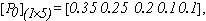
- For the purpose of explaining to the reader the application ofMarkov modelling for predicted rainfall rate, a specific locationis chosen where we divided rainfall rate ranges into five classes starting from zero mm/hr up to the highest rainfall rate asfollows:a. Class A: from zero up to but less than 1 mm/hr.b. Class B: from 1 up to but less than 4 mm/hr.c. Class C: from 4 up to but less than 8 mm/hr.d. Class D: from 8 up to but less than 14 mm/hr.e. Class E: values greater than 14 mm/hr.The discrete time interval chosen in this study was one hour. The reason being that environment should supplyweather data in one hour intervals. However, the method canbe applied for finer grain intervals given that weather data forshorter intervals are available.The approach in grouping total rain conditions into classifiedblocks has been depicted in Figure 1. This classificationin actual data provides the basis for the data required to applyMarkovian theory in the prediction of rainfall rate[8].
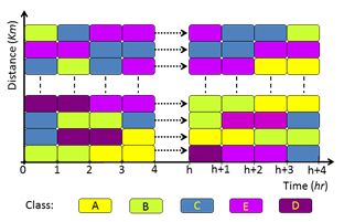 | Figure 1. Presentation of the five rainfall rate classes |
2.1.2. Markov Model Implementation
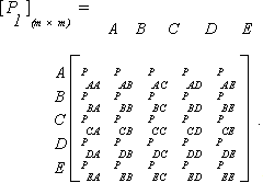
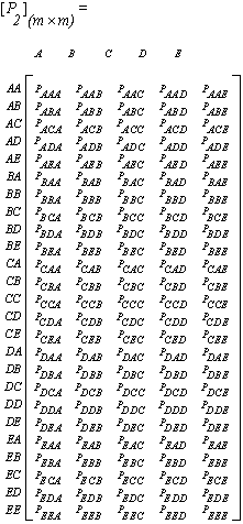
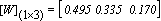
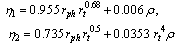
- I- Weight of Transition Probability Matrices:Different weights are assigned to each Markov state, zero order(present state), first order (previous state), and second order(previous to previous state), as defined in Markov Chaintheory. There exist no direct formulas for calculating theseweights and it needs iterative search involving trial and error.The weight values need to be validated over many sets of data.The resulting weight vector is denoted as:
 | (1) |
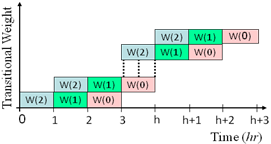 | Figure 2. Presentation of the three different weights |
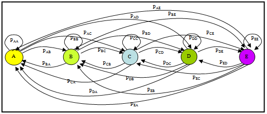 | Figure 3. First Order Markov Chain model with transition probabilities for switching among different states |
 | (2) |
 | (3) |
 | (4) |
2.1.3. Predicted Rainfall Rate
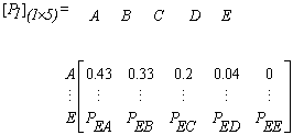
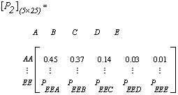
- The value of predicted rainfall rate for the immediately followingdiscrete time period is computed based on probability andweight combinations. These combinations present a specialmodule of weather prediction of different weights assigned toeach transition probability matrix along with Markov Chain oforder , where is finite and equal to 2 in our case. Thus,the prediction of the future state is dependent on the present,previous, and previous to previous states and is independent of the other earlier states[8].Given that the zero [P0], first [P1], and second order [P2] transition probability matrices with the weights assigned to each matrix (W(0)), (W(1)), and (W(2)),respectively. The predicted rainfall rate values can be computed as follows:
 | (5) |
 | (6) |
 | (7) |
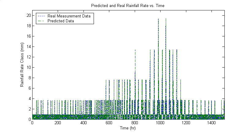 | Figure 4. Comparison of actual and predicted rainfall rate values at South West of King City |
2.1.4. The Values of Weights and Transition Probabilities
- The values of the weight matrix as defined in (1) and the transitionprobabilities as defined in (2), (3), and (4)were obtainedthrough an extensive exercise of iterative adjustments and theirtest of validity on rainfall rate data. At the end, the study notonly revealed a set of workable values but they also revealed the following behaviours:1- For a given set of transition probabilities, there is a correspondingweight that gives the best prediction of rainfallrate in Markov Chain theory.2- Studies done over actual rain data revealed that the fivestates model developed here gives extremely reliable predictionof rain with the following values of weights (W’s)are:
 | (8) |
 | (9) |
 | (10) |
 | (11) |
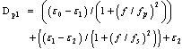
2.2. Migrating ITU-R Model from the Design Domain to the Operational Domain
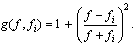
- ITU-R technique for estimating environmental attenuations based on weather data collected over a decade and a half has served us well in system design because it is able to provide average and boundary conditions that a communication system would be subjected to. ITU-R provides not only the geographic parameters of a location, such as the height above the sea level and the average rain height as shown in Figure 5,but also the weather factors like probability of precipitation and mathematicalformula for estimating rainfall rate, and subsequentlyestimatingsignal attenuation due to rain, gas, cloud, fog, andscintillation. The knowledge of the attenuation servesuseful purpose in optimizing the design by finding the best combination of frequency, modulation,coding, and othertransmission and reception parameters for a given location in relative to other locations.
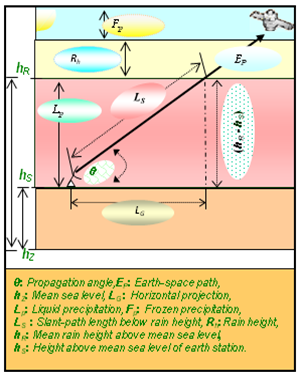 | Figure 5. Earth-space path |
3. Calculation of Rain, Gaseous, Cloud,Fog, and Scintillation Attenuations
- In this paper, a new relationship model is proposed for estimatingvarious weather attenuations as a function of propagationangle, RRpr, and frequency, for any derived geographic locationof ground terminals. This model results in three dimensionalgraphs which relates the attenuation, RRpr, and propagationangle for a selected operational frequency, which may be anyvalue from 0 to 55 GHz. RA is the single greatest weatherdependent signal attenuation factor, which occurs in satellitenetworks largely due to signal absorption and scattering of incomingsignal. Fortunately rain forms only in the tropospherethat extends around sixteen kilometers from sea level whilethe satellites are located in geostationary orbit at 35,800 kmabove earth[6]. Therefore, exposing signal to rain attenuationonly during a small portion of its transmission path as shownin Figure 6.Nevertheless as the frequency increase the losses increaseas shown in Table 2[32]-[35]. Even heavy rainfall of 10 cm/hrseems to cause a small attenuation of 0.05 dB/km with RF signalsat 2.4 GHz. The Ku band attenuation for the same rainfall,however, is approximately nine times that of C-band, andthus very substantial for it to be ignored[36],[37]. Therefore,estimating different atmospheric attenuations at regional or individualsites is important for improving control ofsatellite channel parameters especially when higher transmissionfrequencies are adopted to achieve greater transmissionrate through communication channels.
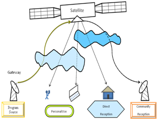 | Figure 6. A satellite broadcast system in the presence of horrendous weather condition |
|
3.1. Calculating Rain Attenuation (RA)
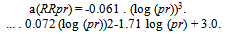
- The RA, represented as (Ar), is predicted by using a set offunctions and solving them for different satellite-location dependentvalues. The values of RA are calculated as a functionof frequency (f) and predicted rainfall rate (RRpr). The foundationalwork of this technique and its variables are explainedin[5],[14] and[38].The key destination of this technique is that we start with anattenuation value at a known frequency (fn), and then estimatethe attenuation at one increment higher frequency (fn+1).Then using the attenuation at (fn+1), we find attenuation at(fn+2), and so on. That is, once RA is known at any lowerfrequency, we will be able to compute RA at a higher frequency andcontinue the process until the maximum desiredfrequency is reached.This iterative calculation is made using the following threeequations. Equation (12) establishes the relationship betweenRA and RRpr(see[13],[19]for full description).Thesecond equation (13) establishes relationship between an intermediatevariable H with a known value of RA at a knownfrequency (fn). Then the next equation (14)calculates RA atthe next frequency (fn+1). This process is iteratively repeateduntil RA reaches the desired frequency. The RA for different frequencies and RRpr values can beobtained from[13]:
 | (12) |
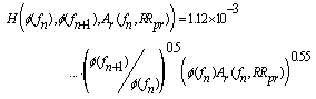 | (13) |
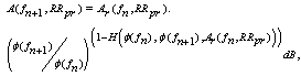 | (14) |
 | (15) |
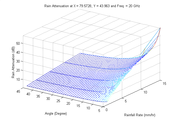 | Figure 7. Rain attenuation at South West of King City |
3.2. Calculating Gaseous Attenuation
- In this section, an analytical method for estimating gaseousattenuation has been presented. This has been an extension ofthe methodology presented in ITU-R P. 676. The slant pathattenuation depends on various meteorological conditions createdby the distribution of temperature, pressure, and humidityalong the transmission path. Thus, the effective path lengthvaries with location, month of the year, height of the stationabove the sea level, and propagation angle. The gaseous attenuationis calculated using the following steps:1.Specific attenuation for dry air (γτ )2.Specific attenuation for water vapour (γv)3.Equivalent path length for dry air (hτ)4.Equivalent path length for water vapour (hv).ematical technique for obtaining the values of theseparameters is given below. The calculation of total gaseousattenuation (Ag), then follows:1. Specific Attenuation for the Dry Air (γτ):The attenuation (dB/km) for the frequency (f≤54 GHz) is given as:
 | (16) |
 | (17) |
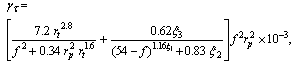 | (18) |
 | (19) |
 | (20) |
 | (21) |
 | (22) |
 | (23) |
 | (24) |
 | (25) |
 | (26) |
 | (27) |
 | (28) |
 | (29) |
 dB,and θ ≤5°. Thus, the estimated gaseous values are computedat any desired location, for all ranges of propagation angle andRRpr, and for any frequency as shown in Figure 8.
 | Figure 8. Gaseous attenuation at South West of King City |
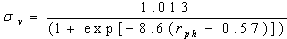
3.3. Calculating Cloud and Fog Attenuations
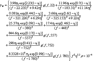
- Cloud and fog can be described as a collection of smaller raindroplets, or alternatively, as different interactions from rain asthe water droplet size in fog and cloud is smaller than thewavelength of 3 GHz signals. The cloud and fog attenuations(Acf) can be expressed in terms of RRpr and propagationangle for a specific frequency and temperature valuestk (Kelvin), through the following series of equations, culminating into equation (37).
 | (30) |
 | (31) |
 | (32) |
 | (33) |
 | (34) |
 | (35) |
 | (36) |
 | (37) |
 | (38) |
 | (39) |
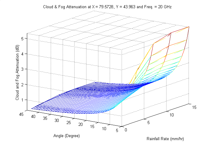 | Figure 9. Cloud and Fog attenuations at South West of King City |
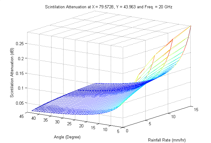 | Figure 10. Scintillation attenuation at South West of King City |
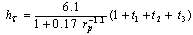
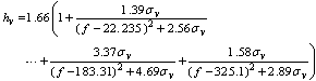
3.4. Calculating of ScintillationAttenuation
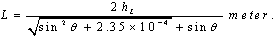
- The cumulative distribution of tropospheric scintillation isbased on monthly or longer average ambient temperature.This distribution reflects the specific climate condition of thesite[5],[39]. In satellite communications, scintillation attenuationresults from rapid variations in the signal’s amplitude andphase due to changes in the refractive index of the earth’s atmosphere.A general technique for predicting this attenuationas a function of RRpr and propagation angle that is greaterthan 4° is given here.Calculate the standard deviation of the signal amplitude,σref as:
 | (40) |
 | Figure 11. Atmospheric attenuation at South West of King City |
 | (41) |
 | (42) |
 | (43) |
 | (44) |
 | (45) |
 | (46) |
 | (47) |
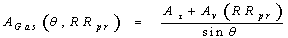
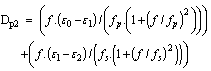
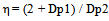
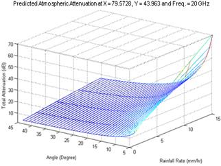
3.5. Calculating Total Attenuation
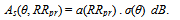
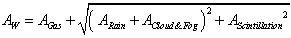
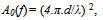
- The total attenuation At is made up of two components:Weather attenuation (AW) and free space attenuation (A0).The weather attenuation (AW) is calculated from the four constituentattenuations calculated in preceding subsections. Theyare:1. Ar(θ, RRpr): rain attenuation, as estimated in (15).2. Ag(θ,RRpr): gaseous attenuation due to water vapourand oxygen, as estimated in (29).3. Acf(θ,RRpr): cloud and fog attenuations, as estimatedin (39).4. As(θ,RRpr): attenuation due to tropospheric scintillation,as estimated in (47).Given these four attenuations, the total weather attenuationAW(θ,RRpr), can be calculated from[5],[8], and[13]:
 | (48) |
|
 | (49) |
 | (50) |
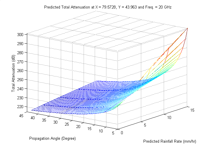 | Figure 12. Predicted total attenuation at South West of King City |
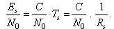
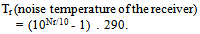
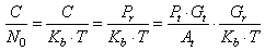
3.6. Relating Total Attenuation with Signal to Noise Ratio (SNR)
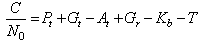
- SNR is a measure of signal strength for satellite signal relativeto attenuations and background noise, usually measuredin decibels (dB)[41]. The signal energy (Es) to noise powerspectral density (N0) per symbol is calculated from the knowledgethat Es = C .Ts = C = Rs, where C is signal power,Ts is symbol duration, and Rs transmission rate.
 | (51) |
 | (52) |
 | (53) |
 | (54) |
 | (55) |
 | (56) |
4. Simulation Results and Discussions
4.1. Simulation Environment and Implementation
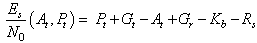
- The mathematical solution for finding any weather attenuationand utilizing that information to improve signal qualityin satellite networks were tested in a simulated system namedIWACS. The system monitors channel qualities and appliescounter measures, which involves controlling of power, frequency,propagation angle, modulation, coding, and data rate.The outcome is the evolution in signal fidelity, especiallyabove 10 GHz, through reduction in digital transmission errors.In this section, the architecture of the IWACS is brieflymentioned. Details are avoided because the material presentedin earlier section has been the main focus of this article.The IWACS was simulated in Matlab simulations version7.10.0 running on i7 - 2630QM, 2.00 GHz CPU and6.00 GB RAM. A special module was written to read weatherdata from Environment Canada supplied in aspecially formattedtext stream and converted into a three hour sliding windowof moving weather data always proceeding the present moment.Software modules were written to extract propagation related parameters shown in Figure 5 for the location from ITURsupplied data. Algorithm for predicting the RR based onMarkov theory with fixed-duration weather data was written.Also, the IWACS used heuristic algorithms that employedfield inputs in problem solving, learning and discovery.The system adhered to formalized knowledge represent ations chemes practiced in the industry, and machine learning techniques,to reach optimal decisionin dealing with differentatmosphericconditions[5],[8],[16],[42], and[43].The key feature of the IWACS is that it adjusts to signalvariations with a fast response time. In accomplishing this, theemployed technique used feedback of SNR values from thereceiving end of the channel and uses that knowledge to mitigatefuture weather attenuations, thus preventing them fromactually manifest in the channels. This proactive approachto the adjustment of signal characteristics is what makes thesystem meet end-to-end QoS requirements.The core architecture of the IWACS is shown in Figure 13,where it may be noted that it consists of four control blocks,the first control block, the second control block, the third controlblock, and the fourth control block, a feedback loop andcounter iteration, along with a special module called decisionsupport system (DSS). This figure illus- trates the Interrelation-shipsof various blocks involved in tuning propagation characteristicsof a communication
 | Figure 13. Intelligent weather aware system for satellite networks |
|
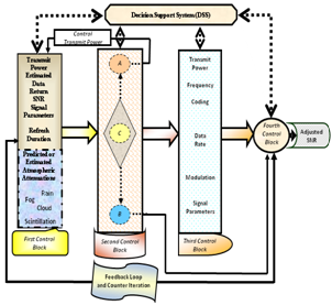
 | Figure 14. Network optimization Decision Support System (DSS) |
4.2. Results
- The system, built on the foundation of the above mentionedprinciples, was found to deliver noteworthy improvements inthe performance of satellite networks. The system monitored the SNR atthe receiving end of the channels, compared it with a threshold,and searched for a blend of available power, frequency,propagation angle, coding, transmission rate, and modulationin response to predicted channel attenuation. It then attemptedto maintain a desired level of SNR as shown in Figure 12, Figure 13, Figure 14,Figure 15, andFigure 16. Such maintenance required the aid of anexpanded form of Table 4 for selecting the right combinationof propagation parameters.Figure 15 and Figure16 compare the SNR before and afterthe techniques discussed in this paper are put to usefor making improved system performance. These figures representcases when SNR fell between (-39 ~-16) dB,and transmit power from (-100 ~ -88) dB before intelligentdecision mechanism was turned on. The improvementsmade in SNR and transmit power level were significant afterthe IWACS was allowed to operate under the same conditions.The SNR improved to (5 ~ 27) dB and the transmit powerlevel ranged from (-63 ~-51) dB.Both cases were subjectedto identical weather conditions where total attenuationdue to weather rangedfrom (215 ~ 225) dB for a frequencyof 20 GHz at 40 degree propagation angle. Note that the systemwas able to bring the upper limit of transmit power to lessthan the maximum allowed of -30 dB. Any time this limitis reached, signal parameters are re-adjusted to prevent uncontrolledsignal transmission as shown in Figure 16and Table 4. Itshould be noted that the improvements in channel performancemade by the scheme are significant.
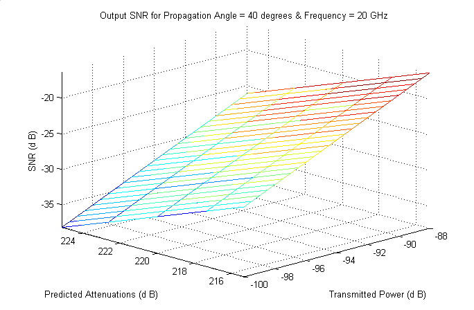 | Figure 15. Output SNR at South West of King City channel |
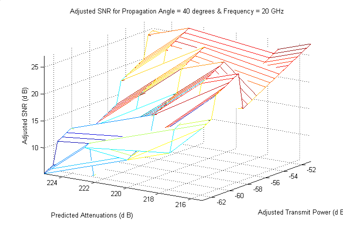 | Figure 16. Adjusted output SNR at South West of King City |
5. Conclusions
- Precipitation, gaseous formation, cloud, fog, and scintillationcause attenuation of satellite signals. These attenuationsbecome especially prominent at frequencies above Ku band.Such attenuation makes it difficult to provide agreed upon QoSby satellite networks unless special mitigation measures aredevised to counter weather effects. Such control systems couldbe optimized to its most effective status if we had the bestpossible techniques for predicting channel attenuation due toweather related factors.This paper presents a technique forpredicting channel attenuation based on real-time weather dataand the use of the Markov theory. The results thus obtained, arefound to be able to make significant improvement over thetechniques known thus far. This technique positively contributesto QoS maintenance by allowing for better tuning andadaptation of signal propagation parameters such as frequency,power, propagation angle, modulation, coding, and transmissionrate with changing weather conditions. The paper also introducesa three dimensional relationship model between attenuation, propagation angle, and RRprwith an implication that for a given atmospheric condition, the signal attenuationcould be predicted with much improved accuracy thanthe techniques known to us. An IWACS, which controls modulation, coding, transmission power, frequency, propagationangle, and transmission rate to improve channel robustness, isbriefly described. It is believed that the technique presentedhere can be of significant interested to research and developmentcommunity interest in improving the throughput of satellitenetworks.
ACKNOWLEDGEMENTS
- This work is supported by the Deanship of Scientific Research (DSR)at King Fahd University of Petroleum & Minerals (KFUPM) through projectNo. JF111005.
References
| [1] | R. K. Crane, “Prediction of the effects of rain on satellite communication systems,” Proc. of the IEEE, vol. 65, pp. 456–474, March 1977. |
| [2] | F. Haidara, A. Dissanayake, and J. Allnutt, “A predictionmodel that combines rain attenuation and other propagation impairments along Earth-satellite paths,” IEEE Trans. on Antennas & Propagation, vol. 45, pp. 1546–1558, Oct. 1977. |
| [3] | ITU-R, Rain height model for prediction methods. Radio wave propagation, International Telecommunication Union. Rec. P.837-4, ITU-R, Fascicle,Geneva, 2001. |
| [4] | D. V. Rogers, L. J. I. Jr., and F. Davarian, “System requirements for ka-band Earth-satellite propagation data,” Proc. of the IEEE, vol. 85, no. 6, pp. 810–820, 1997. |
| [5] | K. Harb, A. Srinivasan, B. Cheng, and C. Huang, “Intelligent weather aware scheme for satellite systems,” in Proc. IEEE ICC’08, May 2008. |
| [6] | J. Pelton, “The start of commercial satellite communications [History of communications],” IEEE Communications Magazine, vol. 48, no. 3, pp. 24–31, 2001. |
| [7] | L. J. Ippolito, “Propagation effects and system performance considerations for satellite communications above 10 GHz,” Proc. of the IEEE, vol. 1, pp. 86–91, Dec. 1990. |
| [8] | K. Harb, F. R. Yu, P. Dakhal, and A. Srinivasan, “Performance improvement in satellite networks based on markovian weather prediction,” in Proc. IEEE GlobCom’10, Dec. 2010. |
| [9] | A. A. Aboudebra, K. Tanaka, T. Wakabayashi, S. Yamamoto, and H. Wakana, “Signal fading in land-mobile satellite communication systems: Statistical characteristics of data measured in Japan using ETS-VI,” Microwave, Antennas & Propagation, vol. 146, pp. 349–354, Oct. 1999. |
| [10] | L. J. Ippolito and T. A. Russell, “Propagation considerations for emerging satellite communications applications,” Proc. of the IEEE, vol. 81, pp. 923–929, June 1993. |
| [11] | L. Mathy, C. Edwards, and D. Hutchison, “Principles of QoS in group communications,” Telecommunication Systems, vol. 11, no. 1-2, pp. 59–84, 1999. |
| [12] | ITU-R, “Attenuation due to clouds and fog,” Radio wave propagation, International Telecommunication Union Recommendation ITU-R P.840-3, 1999. |
| [13] | K. Harb, A. Srinivasan, B. Cheng, and C. Huang, “Prediction method to maintain QoS in weather impacted wireless and satellite networks,” in Proc. SMC, Oct. 2007. |
| [14] | ITU-R, Specific attenuation model for rain for use in prediction methods. Radio wave propagation, International Telecommunication Union. Rec. P.838-3, ITU-R, Fascicle, Geneva, 2003. |
| [15] | K. Harb, F. R. Yu, P. Dakhal, and A. Srinivasan, “A decision support scheme to maintain QoS in weather impacted satellite networks,” in Proc. AIAA Atmospheric and Space Environments Conference’10, (Toronto, ON, Canada), Aug. 2010. |
| [16] | Telesat Canada, “ISS (Intelligent Satellite Service) Research and Development.” website: http://www.telesat.ca, last accessed date March 2012. |
| [17] | J. S. Mandeep, Y. Y. Ng, H. Abdullah, and M. Abdullah, “The study of rain specific attenuation for the prediction of satellite propagation in Malaysia,” Journal of Infrared, Millimeter and Terahertz Waves, vol. 31, no. 6, pp. 681–689, 2010. |
| [18] | ITU, “Radio communiation sector (ITU-R) home.” website: http://www.itu.int/ITU-R, last accessed date April 2012. |
| [19] | K. Harb, A. Srinivasan, B. Cheng, and C. Huang, “QoS in weather impacted satellite networks,” in Proc. IEEE Pacific Rim Conference on Communications, Computers and Signal Processing, (Victoria, B.C., Canada), Aug. 2007. |
| [20] | C. I. Christodoulou, S. C. Michaelides, M. Gabella, and C. S. Pattichis, “Prediction of rainfall rate based on weather radar measurements,” in International Joint Conference on Neural Networks IJCNN, (Budapest, Hungary), July 2004. |
| [21] | J.-C. Hsieh, H.-P. Lin, and C. Yang, “A two-level, multistate markov model for satellite propagation channels,” Proc. IEEE VTC, vol. 4, pp. 3005–3009, May 2001. |
| [22] | J. A. Garcia-Lopez, J. M. Harnando, and J. M. Selga, “Simple rain attenuation prediction method for satellite radio links,” IEEE Trans. on Antennas & Propagation, vol. 36, pp. 444–448, March 1988. |
| [23] | U. C. Fiebig, “Modeling rain fading in satellite communications links,” in Proc. IEEE VTC’99, vol. 3, pp. 1422–1426, Sept. 1999. |
| [24] | E. E. Altshuler, M. A. Gallop, Jr., and L. E. Telford, “Atmospheric attenuation statistics at 15 and 35 GHz for very low elevation angles,” Radio Science, vol. 13, no. 5, pp. 839–852, 1978. |
| [25] | S. D. Slobin, “Microwave noise temperature and attenuation of clouds: Statistics of these effects at various sites in the United States, Alaska and Hawaii,” Radio Science, vol. 17, no. 6, pp. 1443–1454, 1982. |
| [26] | L. Saloff-Coste, Lectures on finite Markov chains. In Lectures on probability theory and statistics (Saint-Flour, 1996), vol. 1665. Springer, Berlin, 1997. |
| [27] | V. Network, “Bilinear interpolation definition.” website: http://www.pcmag.com/encyclopedia-term/0,1237,t=bilinear+interpolation&i=38607,00.asp, last accessed date March 2012. |
| [28] | R. McLeod and M. L. Baart, Geometry and Interpolation of Curves and Surfaces. Cambridge University Press, July 1998. |
| [29] | D. A. Sanchez-Salas and J. L. Cuevas-Ruiz, “N-states channel model using Markov Chains,” Proc. of Electronics, Robotics and Automotive Mechanics Conference, pp. 342 – 347, Oct. 2007. |
| [30] | W. Suozhu, L. Haifang, and H. Zhaohui, “Application of Markov Chains prediction model in product layout optimization,” International Forum on Computer Science-Technology and Applications (IFCSTA)’09, vol. 3, no. 10, pp. 243–246, 2009. |
| [31] | V. Network, “VSAT network types.” website:http://www.comsys.co.uk/wvm mn.htm, last accessed date Feb. 2012. |
| [32] | K. M. S. Murthy, J. Alan, J. Barry, B. G. Evans, N. Miller, R. Mullinax, P. Noble, B. O’Neal, J. J. Sanchez, N. Seshagiri, D. Shanley, J. Stratigos, and J. W. Warner, “VSAT user network examples,” Communication Magazine, vol. 27, pp. 50–57, May 1989. |
| [33] | D. Chakraborty, “VSAT communications networks - An overview,” Communication Magazine, vol. 26, pp. 10–24, May 1988. |
| [34] | L. P. Seidman, “Satellites for wideband access,” Communication Magazine, vol. 34, pp. 108–111, Oct. 1996. |
| [35] | ITU-R, Propagation data and prediction method required for the design of Earth-space Telecommunication systems. Radio wave propagation, International Telecommunication Union. Rec. P.618-7, ITU-R, Fascicle, Geneva, 2001. |
| [36] | L. A. Hoffman, H. J.Wintroub, and W. A.Garber, “Propagation observations at 3.2 millimeters,” Proc. of the IEEE, vol. 54, pp. 449–454, June 2005. |
| [37] | K. Harb, F. R. Yu, P. Dakhal, and A. Srinivasan, “An intelligent QoS control system for satellite networks based on markovian weather,” in Proc. IEEE VTC’08, Sep. 2010. |
| [38] | Y. Karasawa, K. Yasukawa, and M. Yamada, “Tropospheric scintillation in the 14/11-GHz bands on Earthspacepaths with low elevation angles,” IEEE Trans. onAntennas & Propagation, vol. 36, pp. 563–569, March1988. |
| [39] | G. Maral and M. Bousquet, SatelliteCommunicationsSystems. John Wiley & Sons Ltd, UK, 1993. |
| [40] | E. Lutz, M. Werner, and A. Jahn, Satellite Systems forPersonal and Broadband Communications. Springer,New York, 2000. |
| [41] | Y. Leung, Intelligent spatial decision support systems.Springer Verlag, New York, 1997. |
| [42] | L. J. Bannon, “Group decision support systems: An analysis and critique,”In Proceedings of 5th European Conference on Information Systems, pp. 526-539, June 1997. |