J. M. R. de Souza Neto 1, J. J. C. Silva 1, T. C. M. Cavalcanti 1, J. S. da Rocha Neto 1, I. A. Glover 2
1Department of Electrical Engineering, Federal University of Campina Grande, Campina Grande, 58100-000, Brazil
2Department of Electronic & Electrical, Engineering University of Strathclyde, City, Postcode, Scotland
Correspondence to: J. M. R. de Souza Neto , Department of Electrical Engineering, Federal University of Campina Grande, Campina Grande, 58100-000, Brazil.
| Email: |  |
Copyright © 2012 Scientific & Academic Publishing. All Rights Reserved.
Abstract
The practical engineering plausibility of transmission-loss inversion methods using low-cost sensor network technologies for location and tracking of small ruminants is investigated experimentally. Transmission loss is measured in representative outdoor environments using IEEE 802.15.4 technology. The simplest possible propagation model is shown to reflect the general features of the measured propagation data. Its absolute accuracy, however, is probably inadequate for use in a location algorithm based on model inversion without optimization of its parameters. Model calibration to reflect inter-site variation of the propagation environment is suggested as a possible way of realizing a location system with useful accuracy and adequate portability.
Keywords:
Tracking, Location, Transmission Loss Inversion, Animal Husbandry, Wireless Sensor Networks, IEEE 802.15.4, Propagation
Cite this paper:
J. M. R. de Souza Neto , J. J. C. Silva , T. C. M. Cavalcanti , J. S. da Rocha Neto , I. A. Glover , "Low-Cost WSN Monitoring and Location of Small Ruminants Using Transmission-Loss Inversion on Open Grassland in Brazil", Journal of Wireless Networking and Communications, Vol. 2 No. 5, 2012, pp. 101-110. doi: 10.5923/j.jwnc.20120205.04.
1. Introduction
The work reported here is part of a larger project to devise an animal tracking and monitoring system for the investigation of the relationships between the distribution of plant species available to grazing/browsing animals, animal preferences in the species selected, distances travelled to satisfy these preferences and animal health and growth rate. The system will employ sensors fitted to free-ranging, and semi-free-ranging, animals (in the first instance goats) to monitor rate of food ingestion. Real-time communication of the sensor data to an information collection station is to be implemented using IEEE 802.15.4 technology. It is proposed that animal tracking be achieved by measuring received signal strength from transmissions at multiple (at least three) widely separated points on the perimeter of the monitored area. The use of distributed wireless sensors has been discussed for over a quarter of a century. Only relatively recently, however, with advances in the production of low-power, miniaturised electronics have they become truly practical for low-cost applications [1]. Inversion of the transmission-loss range characteristic will then allow location by tri- (or multi-) lateration. Although this location technique is well known in principle its practicality, in terms of achieving useful location accuracy is questionable especially in the context of systems that may be deployed in regions with differing physical characteristics (vegetation cover, composition of soil, humidity etc.) We describe here transmission-loss measurements, using the target technology (IEEE 802.15.4), and its modelling carried out in two different environments and the use of these measurement and corresponding models to assess the plausibility of engineering a practical system with useful accuracy [2, 3].
2. Methodology
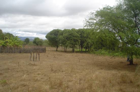 | Figure 1. Location A (Patos-PB) |
Measurements of transmission loss and received signal have made between a pair of omnidirectional antennas in two flat, rural, locations in North-East Brazil which we refer to as Location A (Patos - PB) and Location B (Campina Grande - PB). Location A is typical of those that are used for goat and sheep farming in this region of Brazil, Figure 1. Location B represents short, cropped, grass and is more typical of cultivated pasture that might be used for cattle grazing. Figure 2. Location B is, conveniently, within the campus boundary of Federal University of Campina Grande (UFCG), Figure 3 and Figure 4 are schematic diagrams showing the precise extent of the measurements in relation to their immediate physical environments.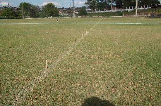 | Figure 2. Location B (Campina Grande-PB) |
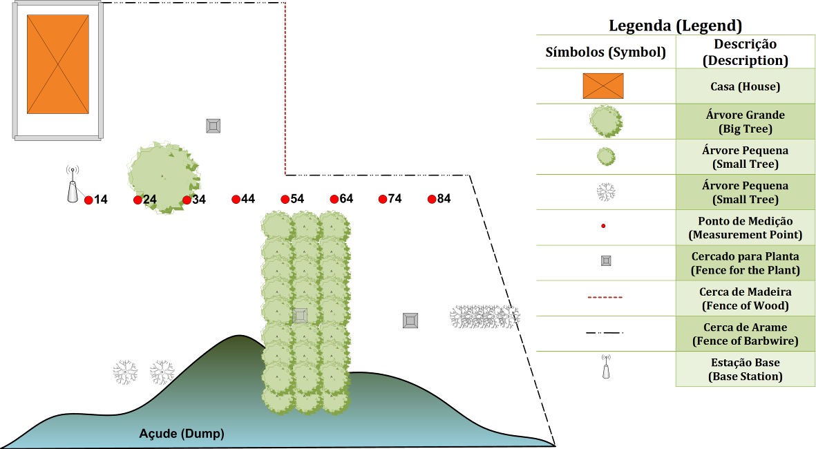 | Figure 3. Measurement locus at Location A |
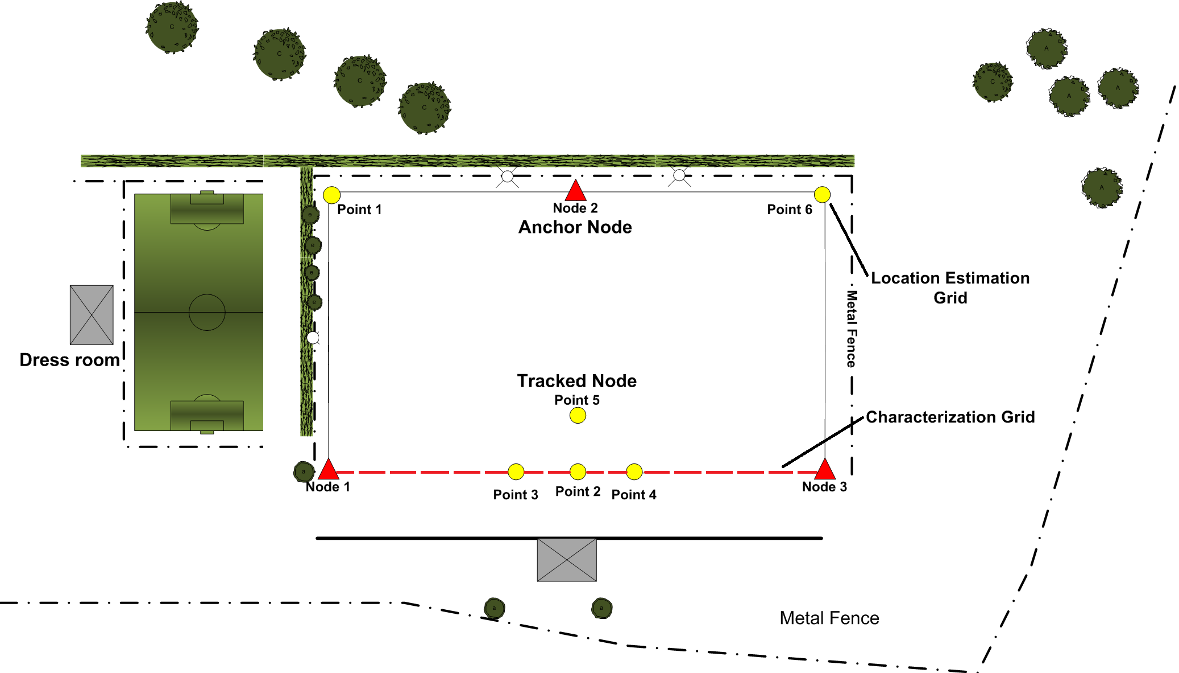 | Figure 4. Measurement locus at Location B |
 | Figure 5. Measurement range superimposed on two-ray transmission-loss model |
The climate of Location A is generally hot (mean winter and summer day-time temperatures 25.8℃ and 30.2℃ respectively [4]). The noncalcic brown soil is sandy and generally dry with high saline-sodic content [5, 6]. The ground cover is predominantly scrub vegetation with occasional small trees. The climate of Location B is slightly cooler (mean winter and summer day-time temperatures 27.6 ℃and 22.3℃ respectively. The soil at Location B has low salinity possibly due to the addition of natural manures. Both measurement locations are part enclosed by a fence (approximately 1.3 m in height).
3. Measurements
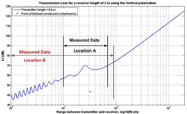
All the measurements in both locations were made using vertically polarized antennas. Propagation modelling can be physical or empirical. The former has been adopted since it has the significant advantage of portability, i.e. a physical model can be deployed in a variety of environments without requiring an extensive set of propagation measurements in each. The simplest plausible physical model for the predominantly flat terrain expected is a two-ray model accounting for direct and ground reflected paths. The path-length measurement range was therefore selected to span the break point in this model between the quasi-periodic interference pattern expected for distances less than that corresponding to the farthest point of constructive interference and the monotonic pattern expected beyond this point, Figure 5.This is because agreement between theory and experiment in this region would be good evidence of the adequacy of the two-ray model that could then be extrapolated. The path-length (R) corresponding to the farthest point of constructive interference is given by [7]: | (1) |
where ht and hr are transmitter and receiver heights respectively and λ is wavelength. IEEE 802.15.4 technology uses the unlicensed ISM frequency band for 16 channels between 2.4 and 2.4835 GHz corresponding to a wavelength between 12.07 and 12.49 cm. The protocol allows dynamic channel selection (a scan function that steps through a list of supported channels in search of a beacon) and, using receiver energy detection, yields a link quality indication. The height of the transmitter was 0.5 m and the height of the receiver was 2.0 m at Location A. The height of both transmitter and receiver was 1.0 m at Location B.
3.1. Location A Measurements
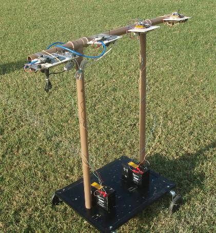
Data Set A comprises a line of high-resolution (20 cm) received signal strength indication (RSSI) measurements. The minimum path-length of the measurements was 10.0 m and the maximum path-length was 70.0 m. The measurement locus is marked by the (red) dotted line (measurement points 24 to 84) in Figure 3. In order to accelerate the measurement process five transmitter modules, with the required 20 cm spacing, were mounted on a 1.0 m horizontal spacing bar, Figure 6, allowing multiple measurements to be recorded simultaneously.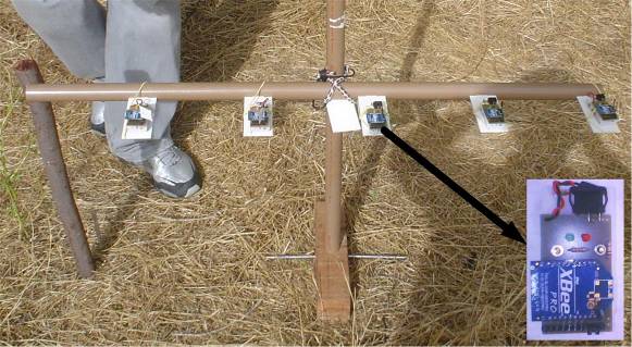 | Figure 6. Multiple transmitters mounted on spacing bar – Location A measurements |
This is possible since each received data packet identifies its originating node. The spacing bar was made of PVC to minimize the effect of scattering. For each path-length the RSSI for up to 150 packets was logged. Corrupted packets were discarded and the mean value of all remaining received powers was calculated. In the event that less than 100 uncorrupted packets were received the data point was replaced by the spatial mean of the data points on either side. Such interpolation was required for 9.7% of the data.The output power (Pt) of all five transmitting nodes was set to the nominal value of 3.6 dBm. The effect of small differences in radiated power due to deviations from the nominal value was removed using the data pre-processing algorithm: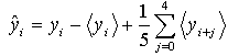 | (2) |
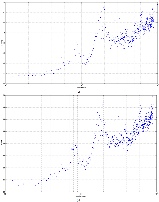
where yi is the received power from the ith transmitted packet and  denotes mean value (taken over a minimum of 100 packets). The raw and processed data are shown in Figure 7(a) and Figure 7(b) respectively.
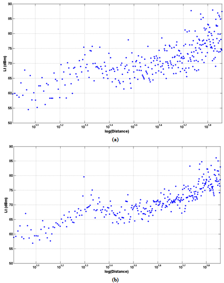 | Figure 7. Location A data set, 7(a) Raw data, 7(b) Pre-processed data |
 | Figure 8. Multiple transmitters mounted on spacing bar – Location B measurements |
 | Figure 9. Location B data set, 9(a) Raw data, 9(b) Processed data |
3.2. Location B Measurements
Data Set B comprises a line of measurements with slightly lower spatial resolution (25 cm) than Data Set A. These measurements are marked by the (red) dotted line in Figure 5. The minimum path-length of the measurements in set B was 25 cm and the maximum path-length was 90.0 m. Four transmitter modules, with the required 25 cm spacing, were mounted on a 1.0 m horizontal spacing bar, Figure 8, allowing multiple measurements to be recorded simultaneously.For each path-length RSSI for up to 500 packets was logged. Corrupted packets were discarded and the mean value of all remaining received powers was calculated. The output power of all four transmitting nodes was set to the maximum nominal value of 18 dBm. The raw and pre-processed data is shown in Figure 9(a) and Figure 9(b) respectively.
4. The Physical Transmission-Loss Model
The simplest possible physical model for propagation over a plane-earth postulates two propagation paths, or rays; a direct line-of-sight ray (d1) and a ground-reflected ray (d2), as shown in Figure 10.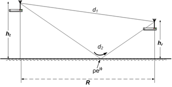 | Figure 10. Two-ray propagation model |
The strength of the ground-reflected signal depends on the antenna beamwidths, the link geometry (link length and antenna heights), the electrical characteristics and the smoothness of the ground at the point of reflection. A complex reflection coefficient, (ρejφ) can be defined such that ρ is the ratio of reflected-wave field-strength magnitude to incident-wave field-strength magnitude and φ is the phase advance which occurs on reflection. The plane surface reflection coefficient for an incident-field polarized parallel to the plane of incidence (i.e. ‘vertical’) is given by the Fresnel equation [8], as shown in Equation (3):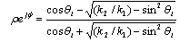 | (3) |
where k1 and k2 are the propagation constants appropriate to the media on the incident and transmission sides, respectively, of the reflecting surface, and θi is the incidence angle. Since the incident medium is air, then k1 = 2π/λ where (to a very close approximation) λ is the free-space wavelength. The square of the complex propagation constant (k) is given by: | (4) |
where ω (=2πf) is angular frequency, ε is permittivity, µ is permeability and σ is conductivity of the middle. The effective reflection coefficient, ρef, for a surface that is not perfectly plane is that given by (3) reduced by the Rayleigh roughness factor (r) [9]: | (5) |
Which accounts for energy lost from the specularly reflected wave due to diffuse scattering. Assuming that the angles of departure and arrival of the ground-reflected ray, at transmitter and receiver respectively, are small compared to the beamwidths of the antennas (such that there is no significant reduction in antenna gain due to the off-axis propagation path of the reflected ray) then the field-strength (F) at the receive antenna will be changed from that when no reflection is present by the factor: | (6) |
The transmission loss (Lt) in decibels is then given by: | (7) |
where Gt and Gr are the (power ratio, not decibel) gains of transmit and receive antennas, respectively. The received signal strength (Pr) is then given by: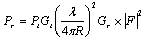 | (8) |
The simple transmission loss model represented by equations (3) - (7) with Gt = Gr = 1.5, s = 3.0 cm, σ = 0.2 and εr = 15 (the electrical parameters recommended in [10] corresponding to medium dry soil) is superimposed on the pre-processed data for Location A in Figure 11.The general features of the data are generally well represented by the model but the parameters used are clearly not optimum in terms of representing the data with minimum error. Some of the discrepancy between model and data might be explained by unaccounted losses (e.g. mismatches between transmitter/receiver and antenna, polarization losses due to imperfect antenna alignment with vertical, reduced antenna directivity due deviation of the monopoles from resonant length and/or a poor ground-plane, and ohmic losses).In terms of assessing the plausibility of the transmission loss inversion based location such unaccounted losses justify a constant offset of the received signal level (and therefore transmission loss) being introduced to improve the agreement of the experimental data with the model.The possibility of path length measurement errors also exists. Again, in terms of assessing the plausibility of the transmission loss inversion technique an error giving the closest agreement with the model can be assumed. Optimization of a constant offset in transmission-loss (4.7 dB) and distance (0.96 m) gives the improved fit between model and data shown in Figure 12.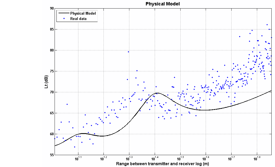 | Figure 11. Comparison of two-ray model with raw data for Location A (εr = 15 and σ = 0.2, s = 3 cm) |
 | Figure 12. Comparison of two-ray model with pre-processed data for Location A incorporating optimum offset in both transmission loss and range (εr = 15 and σ = 0.2, s = 3 cm) |
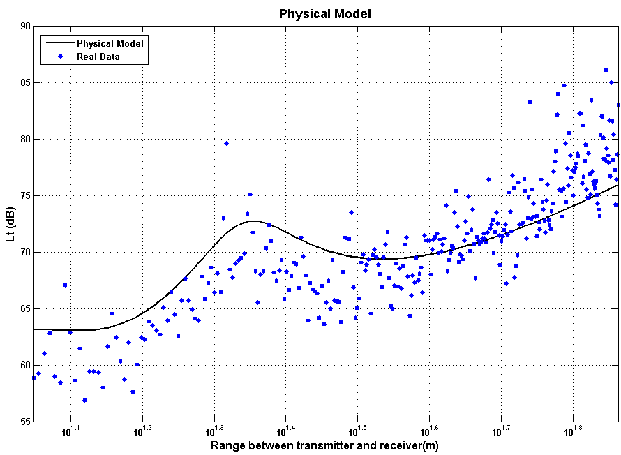
 | Figure 13. Comparison of two-ray model with pre-processed data using optimum offsets (transmission loss and range), s = 3 cm, and optimum electrical parameters (εr = 18.3 and σ = 7.25 S/m) |
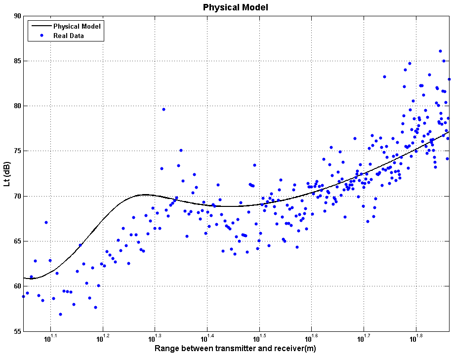
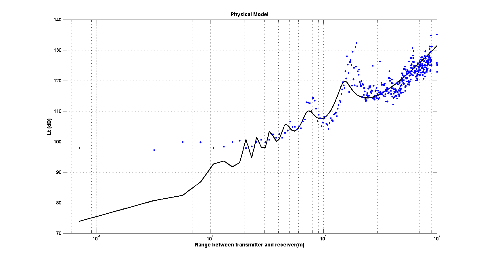 | Figure 14. Comparison between data set and physical model with offset and electrical parameters optimization (εr = 4.77 and σ = 0.896 S/m) |
The RMS error after incorporating both transmission loss and range offsets is 4.0 dB. The error between the model and data can be reduced further by optimizing the electrical parameters of ground. This changes the shape of the curve allowing it to reflect the steepening gradient of the data at large range. Figure 13 shows the model with optimized electrical parameters εr = 18.33 and σ = 7.25 S/m. The RMS error after electrical parameter optimization is 3.2 dB.The same modelling process applied to the measurements taken in Location A was applied to the measurements taken in Location B using Gt = Gr = 1.5 and s = 3.0 cm but with σ = 0.6 and εr = 20. The electrical parameters in this case are those recommended in [10] for medium wet soil reflecting Location B conditions during the measurements. The transmission loss and range offsets required to minimize RMS error between data and model were found to be 7.58 dB and 0.63 m respectively. The transmission loss RMS error after incorporating the transmission loss offset and range offset was 3.95 dB.The error between the model and data can be reduced further by optimizing the electrical parameters of ground. This changes the shape of the curve allowing it to reflect the steepening gradient of the data at large distance. Figure 14 shows the model with optimized electrical parameters εr = 4.77 and σ = 0.896 S/m. The RMS error after electrical parameter optimization is 3.80 dB.The agreement between the data and the two-ray model in Figure 13 and Figure 14 seems reasonable and, superficially, this may be sufficient to encourage further investigation of a location algorithm based on a two-ray model inversion. The real issues, however, are (i) the large intra-site spread of data about the transmission loss law, even after optimization has been carried out to reduce this, and (ii) the non-monotonic nature of the transmission loss law. Both the large data spread (combined with the relatively small gradient of the transmission loss law) and the non-monotonic nature of the law means that a given measurement of transmission loss the potential error in range is large. This problem is compounded when the uncertainty in the electrical parameters of the ground is considered which results in inter-site variation of the optimum transmission loss law. It seems clear from the measurements reported here, therefore, that transmission loss inversion using a physical model alone does not represent a plausible approach to locating a mobile IEEE 802.15.4 node, at least using a modest number of receiving measurement nodes. If a sufficiently large number of measurements is used then it may be possible to effectively average out intra-site range errors and remove outlying ranges estimates that occur due to the non-monotonic nature of the law. This, however, would not address the intra-site variation requiring, essentially, the transmission loss law to be established for each site. The number of measurements required is also likely to mitigate against a low-cost solution.All the above issues suggest that for a practical system with useful accuracy a self-calibrating network of measurements is required. A simple and rapid model calibration process can almost certainly be devised. If a small proportion of the measurement (surveyed) nodes were distributed evenly through the monitored region then measured transmission loss between measurement nodes could be used to derive the transmission loss law. Such a self-calibrating system is currently under investigation.
5. Conclusions
As part of a larger project this results shows us only the modelling of the transmission loss associated to grassland areas used to grazing/browsing animals in Brazil. Propagation measurements have been undertaken to investigate the plausibility of a location system for the monitoring of free-ranging small ruminants based on IEEE 802.15.4 technology, multiple receiving nodes, the inversion of a transmission-loss model and multilateration. A simple two-ray model appears to reflect the general features of measurements well, but an empirical adjustment of the model parameters is generally required. The essential problem is the large spread of data about the path-loss model – even after optimisation of the model parameters. The relatively small gradient of the transmission–loss law relative to the spread means that small variations in received signal strength result in large variations in estimated range. The non-monotonic nature of the two-path law (which is certainly appropriate since interference pattern caused by direct and reflected waves is clearly visible in the data) also results in range ambiguity for some measurements. It is suggested that multilateration using more than three receivers will reduce the errors and that non-linear filtering of the resulting location estimates may be able to identify, and eliminate, estimate outliers, further improving accuracy. If too many receivers are necessary to achieve useful location accuracy, however, then the low-cost advantage of the system will be compromised. These issues are currently being investigated further. In the meantime we believe practicality of a low-cost location system based on simple WSN technology and path-loss inversion remains plausible but unproven.
ACKNOWLEDGEMENTS
The authors would like to thanks to CNPq (Conselho Nacional de Desenvolvimento Científico e Tecnológico - Brasil) and CAPES (Coordenação de Aperfeiçoamento de Pessoal de Nível Superior - Brasil) for financial support of this work.
References
| [1] | Mao, G. and Fidan, B. "Localization Algorithms and Strategies for Wireless Sensor Network", (ISBN978-1-60566-396-8, 978-1-60566-397-5), Information Science Reference, 2009. |
| [2] | Neto, J. M, Silva, J. J. C., Cavalcanti, T. C. M., Rodrigues, D. P., Neto, J. S., Glover, I. A., “Propagation measurements and modeling for monitoring and tracking in animal husbandry applications”. In: International Instrumentation and Measurement Technology Conference., 2010, USA:[s.n.]. |
| [3] | Neto, J. M. R. de S.; Neto, J. S. da Rocha; Yang, Y.; Glover, I. A.; , "Plausibility of practical low-cost location using WSN path-loss law inversion,"Wireless Sensor Network, 2010. IET-WSN. IET International Conference on, vol., no., pp.260-265, 15-17 Nov. 2010 doi: 10.1049/cp.2010.1064URL:http://ieeexplore.ieee.org/stamp/stamp.jsp?tp=&arnumber=5741106&isnumber=5741058 |
| [4] | National Institute of Meteorology (Instituto Nacional de Meteorologia – INMET), (in portuguese: Normais Climatológicas) (1961-1990). Ministério da Agricultura, Pecuária e Abastecimento, 2009. |
| [5] | Brazilian Enterprise for Agricultural Research (Empresa Brasileira de Pesquisa Agropecuária – EMBRAPA), (in Portuguese: Embrapa Solos, UEP Recife, 2006 (Avaliable from: www.uep.cnps.embrapa.br/solos/index.html). |
| [6] | L. N. V. de Andrade, and D. E. Cruciani, Condutividade hidráulica no processo de eluição em um solo bruno-não-cálcico. Sci. agric.[online]. 1996, vol.53, n.1[cited 2009-10-23], pp. 43-50. Available from:. ISSN 0103-9016. doi: 10.1590/S0103-90161996000100006. |
| [7] | I. A. Glover and P. M. Grant, “Digital Communications”, 3rd ed., ISBN 978-0-273-71830-7, Pearson, 2010. |
| [8] | Hecht, Eugene: Optics, 4 th ed., Addison Wesley, ISBN 0-321-18878-0, Pearson, 2002. |
| [9] | Beckmann and A. Spizzichino, The Scattering of Electromagnetic Waves from Rough Surfaces. Norwood, MA: Artech House, 1987, pp. 80–98. |
| [10] | International Telecommunication Union/ITU Radiocommunication Sector ITU-R P.527-3: Electrical Characteristics of the Surface of the Earth, 1992. |
 Abstract
 Reference
 Full-Text PDF
 Full-Text HTML