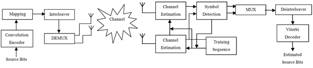
-
Paper Information
- Previous Paper
- Paper Submission
-
Journal Information
- About This Journal
- Editorial Board
- Current Issue
- Archive
- Author Guidelines
- Contact Us
Journal of Wireless Networking and Communications
2012; 2(4): 66-76
doi: 10.5923/j.jwnc.20120204.06
Capacity Analysis of MIMO Spatial Channel Model using Novel Adaptive Semi Blind Estimation Scheme
 Abstract
 Reference
 Full-Text PDF
 Full-Text HTML
Ravi kumar , Rajiv Saxena
Department of Electronics and Communication Engineering, Jaypee University of Engineering and Technology, Guna, India
Correspondence to: Ravi kumar , Department of Electronics and Communication Engineering, Jaypee University of Engineering and Technology, Guna, India.
| Email: |  |
Copyright © 2012 Scientific & Academic Publishing. All Rights Reserved.
Multiple Input Multiple Output (MIMO) has been remained in much importance in recent past because of high capacity gain over a single antenna system. In this article, analysis over the capacity of the MIMO channel systems with spatial channel has been considered when the channel state information (CSI) is considered imperfect or partial. The dynamic CSI model has also been tried consisting of channel mean and covariance which leads to extracting of the channel estimates and error covariance. Both parameters indicated the CSI quality since these are the functions of temporal correlation factor, and based on this, the model covers data from perfect to statistical CSI, either partial or full blind. It is found that in case of partial and imperfect CSI, the capacity depends on the statistical properties of the error in the CSI. Based on the knowledge of statistical distribution of the deviations in CSI knowledge, a new estimation approach which maximizes the capacity of spatial channel model has been tried. The interference interactively reduced by employing the iterative channel estimation and data detection approach.
Keywords: MIMO Capacity, Blind Channel Estimation, Semiblind Channel Estimation, Partial CSI, Spatial Channel
Article Outline
1. Introduction
- MIMO antenna systems is an advanced technique for high data rate transmission over frequency selective fading channels due to its capability to combat the inter-symbol interferences (ISI), low complexity, and spectral efficiency. Information theoretic results show that MIMO systems can offer significant capacity gains over traditional Single Input Single Output (SISO) channels. Using multiple antennas known as MIMO technology, at both the transmitter and receiver, results in further increase in the capacity, provided that the environment is rich scattering. It obtains high data spectral efficiencies by dividing the incoming data into multiple streams and transmitting each stream using different antenna. At the receiver end, these streams are received and separated by various techniques. However, recent works have proposed space-time architecture that simultaneously achieves good diversity and multiplexing performance. This increase in capacity is enabled by the fact that in rich scattering wireless environment, the signals from each individual transmitter appear highly uncorrelated at each of the receive antennas.When conveyed through uncorrelated channels between the transmitter and receiver, the signals at the receiver responds to each of the individual transmitter to separate the signals originating from different transmit antennas.One of the prominent technology being used nowadays is multiple input multiple output orthogonal frequency division multiplexing (MIMO-OFDM) technology to boost the capacity. The multipath characteristic of the environment causes the MIMO channel to be frequency selective for higher data rate transmission. Due to the unique feature of OFDM for converting a frequency selective channel into a parallel collection of frequencies, the receiver complexity is reduced. However to obtain the promised capacity and to achieve maximum diversity gain, MIMO-OFDM system requires accurate channel state information (CSI) at the receiver, in order to perform coherent detection, space-time decoding, diversity combining, and the spatial interference suppression.[1] When using multiple antennas, the coherence distance represents the minimum distance in space separating two antennas such that they experience independent fading.[2]Due to scattering environments, the channel exhibits independent or spatially selective correlated fading which results in lower achievable capacity of MIMO. In MIMO-OFDM systems, channel estimation based on either least squares (LS) or minimum mean square error (MMSE) methods has been widely explored and several estimation schemes have been proposed.[3]Channel estimation based on adaptive filtering has been proposed as an appropriate solution for estimating and tracking the time-varying channel in mobile environments.
2. Constant MIMO Channel Capacity
- When the channel is constant and known perfectly at the transmitter and the receiver, Telater[4] showed that the MIMO channel can be converted to parallel, non-interfereing SISO channel through a singular value decomposition (SVD) of the channel matrix. Waterfilling the transmit power over these parallel channels whose gains are given by the singular values
 of the channel matrix leads to the power allocation
 | (1) |
 is the power in the
  eigenmode of the channel, (x)+ is defined as the maximum of (x,0) and
  is the waterfill level. The channel capacity can be as shown-
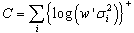 | (2) |
3. Capacity with Partial CSI
- There has been much evolution in the capacity of multiple antenna systems with perfect Channel state information at receiver (CSIR). For multiple antenna systems, the capacity improvement using partial Channel state information at transmitter (CSIT) is under research by so many researchers like Madhow and Visotsky[6], Trott and Narula[7], Jafar and Goldsmith[8-9], Jorswieck and Boche[10] and Simon and Moustakes[11].A full rank matrix is required to generate optimum input covariance matrix which can be incorporated in vector coding across the antenna array. It has been shown in[8] that lower complexity implementation of the vector coding strategy is possible by transmitting several scalar codewords in parallel, without the loss of capacity. It is required to see the transmitter optimization and the optimality of beamforming in the MIMO systems. When a Multiple Input and Single Output (MISO) channel is considered whose channel matrix is rank one, with perfect CSIT and CSIR, it is possible to identify the non-zero eigenmode of the channel accurately and beamforming along the mode. Whereas, with no CSIT and perfect CSIR, Foschini and Gans[12] and Telatar[4] showed that optimal input covariance matrix is a multiple of identity matrix hence the power is equally distributed in all directions. Visotsky and Madhow[6] numerical results indicate that beamforming is close to the optimal strategy when quality of feedback improves. Also Narula and Trott[7] showed that there are cases for mean feedback conditions where the capacity is actually achieved via beamforming for two transmit and receive antenna. A generalized form for optimality of beamforming was given by Jafar and Goldsmith[9] for both cases of covariance and mean feedback.With MIMO antenna systems, the covariance feedback case with correlation at transmitter is solved by Jafar and Goldsmith[13] whereas Jorsweick and Boche[10] implemented the fade correlation at the receiver also. The mean feedback case with multiple transmit and receive antennas was solved by Jafar and Goldsmith in[8] and Moustakas and Simon in[11]. It has been shown that the channel capacity grows linearly with minimum number of antennas either at transmitting and receiving side by Foschini and Gans[12]. This linear increase occurs whether the transmitter knows the channel perfectly (perfectly CSIT) or doesn’t know the channel (no CSIT) at all[4]. Cui and Tellambura in[14] have discussed about the Maximum-likelihood (ML) semiblind gradient descent channel estimator which detects the semiblind data for Rayleigh and Rician channel exploiting the channel impulse response. Feng and Swamy in[15] derived the blind constraint from the linear prediction of MIMO-OFDM with the weighting factor in the semiblind cost function. Abuthinien, Chen and Hanzo in[16] proposed a joint optimization with repeated weighted boosting search of unknown MIMO channel and ML detection of the transmitted data. Expectation maximization algorithm for single carrier MIMO using overlay pilots has been proposed by Khalighi in[17]. Rather than using real input signals, complex input signals have been analyzed by Yu and Lin in[18] using forward-backward averaging method in semi blind channel estimation of space time coded MIMO with zero padding OFDM. Advantage of periodic precoding, block circulant channel model design after cyclic prefix removal and optimal design of precoding sequence has been done by Sheng in[19] for the robustness of the channel estimation w.r.t. channel order overestimation and identification ability of full rank matrix. Analysis of second order statistics of the signal received through sparse MIMO channel exploiting the most significant taps(MST) of the sparse channel forming the correlation matrices of the received signal has been done by Feng in[20]. Better Bit error rate (BER) has been tried recently by Kyeong jin in[21] by designing new iterative extended soft recursive least square(IES-RLS) estimator for both joint channel and frequency offset estimation. Recent work[14-21] has shown the analysis of Mean Square error (MSE) and BER generally without the discussion over capacity analysis, which has been discussed in this paper. Lapidoth and Moser[22] compared with the Zheng and Tse model for block fading[23-24] and showed that without the block fading assumption, the channel capacity in absence of CSI grows only double logarithmically in SNR.By using the channel correlations, the channel matrix components are modelled as spatially correlated complex Gaussian random variable that remains constant for a coherence interval of T symbol period after which these change to another independent realization based in the spatial correlation model. It is shown by Jafar and Goldsmith[25] that the channel capacity is independent of the smallest eigenvalues of the transmit fade covariance matrix as well as the eigenvectors of the transmit and receive fade covariance matrices (QT and QR are the covariance matrix of transmitter and receiver respectively). By looking into the results for the spatially white fading model where adding more transmit antenna beyond the coherence interval length (MT>T) doesn’t increase capacity. Jafar showed that increase in transmit antenna always increase capacity as long as their channel fading coefficients are spatially correlated. It has been shown that with the channel covariance information at the Transmitter(Tx) and Receiver(Rx), transmit fade correlations can be beneficial in the condition of highly mobile and inaccurately measurable fast fading channel by minimizing the spacing between the antenna. It has been shown by an example that with coherence time T=1, the capacity with MT transmit antennas is
 dB higher for perfectly correlated fades than for independent fades.
4. System Model
- A MIMO-OFDM system has been considered with
 transmit antenna and
  receive antenna as shown in Figure 1, which communicates over a flat fading channels, and is abbreviated as
  receive MIMO systems matrix H. The system is described by
 , where x is
  which is the transmitted symbol vector of
  transmitter with the symbol energy given by
  for
for  and covariance matrix
 , y denotes the received vector
  and
and  is the complex valued Gaussian white noise vector at the receiving end for MIMO channels with energy
  distributed according to Nc
  assumed to be zero mean, spatially and temporally white and independent of both channel and data fades. The channel model considered here denoted by
  [26] with
  representing the normalized transmit and receive correlation matrices with identity matrix. The entries of
  are independent and identically distributed (i.i.d.) Nc (0,1).Here the CSIR is described by
  | (3) |
 is the estimate of
  and
and  is the overall channel estimation error matrix,
  are white matrices spatially uncorrelated with i.i.d. entries distributed according to
  with variance
  of channel estimation error.[27].If it is assumed that the system is having lossless feedback, i.e., CSIT and CSIR both are same. Thus
  represents that the CSI is known to both the ends. With the partial CSI model, the channel output can be considered as
  with the total noise given by
  with mean zero and covariance matrix given by
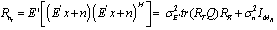 | (4) |
 . It is known that
  is not gaussian and it is not easy to obtain the exact capacity equation. Thus tight upper and lower bounds can be taken in consideration for system design.The mutual information with partial CSI for unpredictable capacity with Gaussian distribution can be denoted as
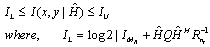 | (5) |
 | (6) |
 denote the lower and upper bounds on the maximum achievable mutual information with the expectation
  considered over the distribution of x. The lower bound capacity (5) has been considered for design criteria. To obtain the highest data rate using the capacity lower bound i.e., to get the best estimates out of all received data estimates, the following problem is required to be solved[27],
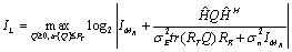 | (7) |
 with the expectation w.r.t. the fading channel distribution. The average SNR of the system is defined as
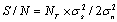 | (8) |
 for
for .
. | (9) |
 is the
  complex valued weight vector of the mth spatial equalizer. The MMSE solution for the NT spatial equalizer considereing the channel to be perfectly known can be shown by
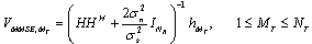 | (10) |
 | Figure 1. Block diagram for the blindly estimation of transmitted symbols using the MIMO systems |
 denotes the mth coloumn of the channel matrix H. It is known that in spatial domain, the short term power is applicable i.e., no temporal power allocation can be considered. On the other hand it is known that the power constraint is applicable across each antenna at each fading state for a given
 . The expectation of mutual information over fading channel distributed can be maximized by maximizing the mutual information[28] i.e.
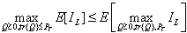 | (11) |
5. Proposed Method
- When the transmitter is considered for both spatial pre-filtering matrix and power allocation, the mutual information of the MIMO system corresponding to nth subcarrier is given by[29], as
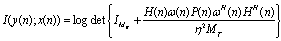 | (12) |
 is the spatial pre filter matrix and power allocation. Assuming the pilot symbols be J which can be denoted as
  and
and  as the available training data. The channel estimation of the MIMO channel pilots J using least square method relies upon
 , which gave us,
 | (13) |
 | (14) |
 should have full rank. To achieve this, choosing
  i.e., assuming
  which can be treated as the lowest number of pilot symbols.The MMSE solution gave the spatial equalizer weight vectors using roughly estimated value
  of channel,
 | (15) |
 denotes the mth coloumn of the estimated channel matrix
 . The weight vectors (15) are not sufficient to estimate correctly because the pilot symbols are in sufficient. It is not easy to use direct decision adaptation, hence a new adaptive method has been proposed. Assuming the data segment of size M i.e. estimated data vector size is M+N-1, where N is the length of the Inter symbol interference (ISI) channel. It is required to calculate
  branch metric which can be calculated by following relation of unknown estimates sequence to avoid sacrifice of tracking ability of channel i.e.,
 | (16) |
 and
and  is the reference channel which is an ideal ISI free channel of the same standards and span length as the blindly estimated channel.Consider (L+1) bits transmitted through an ISI channel of length 2(using Jake’s model) in which L samples which contains the desired block of information. Now it is required to process M samples from these L samples of information by moving one sample forward in each step for getting the M size segment vector. By doing so, we have k processing steps which equal L-M+1 as shown in Figure 2.
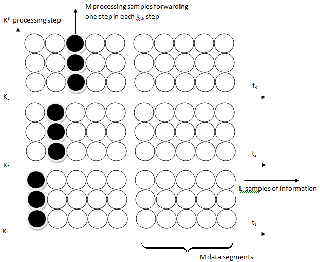 | Figure 2. Proposed channel estimation method |
 for k steps followed by calculating the path metric for all possible paths from the values in matrix
  Now choosing the path with minimum path metric or gain
 and track the bits through the path which will be considered as detected sequence. Now take a short time average value of the detected sequence, i.e.,
 | (17) |
 for all possible estimated vector gives us the selected estimates with minimum branch metric
 . This unique set of selected estimates with minimum
  can be processed further to track surviving states with minimum value from the matrix
  and eventually the possible block of transmitted sequence.To implement this proposed method with (15), we assume the weight vector of mth spatial equalizer with output at sample k as
 . As discussed above,
  where
where  denotes the weights for the mth step which corresponds to the M samples from the L samples of information. Now
  will be processed one sample forward resulting
 , where i denotes the one step forwarding of each weight vector. Calculating the branch metric R for k steps followed by calculating the path metric for all possible paths.
 | (18) |
 is updated at each step using number of iterations which gives the minimum required pilot symbols to detect the signal in a semiblind manner. This updating process of weight vectors has been utilized here from[30]. Since M-QAM modulation has been employed, the complex values will be divided in M/4 regions, each containing four symbol points as
 | (19) |
 . If the spatial equalizers output is dependent on
 , marginal Probability Density Function approximation has been given by[31-32].
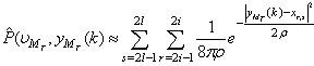 | (20) |
 .Now considering the forwarded step of weight
 , which has been updated as,
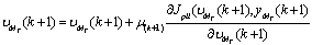 | (21) |
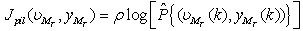 , in which the log of the marginal probability distribution function (PDF) is to be maximized using a stochastic gradient optimization[31-32] and
 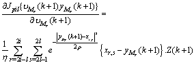 | (22) |
 We have to maintain the value of ρ less than 1 since minimum distance between two neighboring constellation point is 2, which will further ensure the power separation of the four clusters of
 . If the value of ρ is chosen less, then the algorithm may tightly control the segment size and may create problem in identifying the proper estimates. On the other hand, on increasing the value ofρ, degree of separation may not be achieved desirably. For higher SNR conditions, small value of ρ is required whereas for lower SNR conditions, larger ρ is required since the value of ρ is related to the variance which is
 . After receiving the information received by the use of pilot symbol in the form of initial weight vector (15), if it is compared with the pure blind adaptation case as in[31-32], smaller value of ρ can be used which also gives us the study performance. Alternative estimation is also considered in region(19) that includes
 , i.e. single hard estimation, where q denotes the quantization operator and each arriving estimate is weighted by an exponential term, which is a function of the distance between the equalizer’s calculated output
  and the arriving estimate
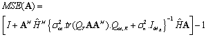
 . This interactive calculation by equalizer will substantially reduce the risk of propagation error and also gives fast convergence, compared with[31]. The capacity analysis after enhancing the estimate perfection leads to get the optimized covariance matrix Q for which we assume an adaptive precoder and decoder(A,B) at the transmitter and receiver end. The received vector after the decoder is given by
 . For MSE, eqn.(7) can be written as
  | (23) |
 | (24) |
 and A. Here
  and
and  are the covariance matrices for the transmitter and receiver. By solving B for Lagrange multiplier associated with the sum power constraint, the problem in (23) can be formulated as
  | (25) |
 | (26) |
 , a Frobenius norm of radius
 . The objective function of (25) is continuous at all points of the feasible set. According to Weierstrass theorem, a global minimum for (25) has been evolved which also exists for(23). Based on the identity for the relation between Lagrange multiplier and receive decoder, MSE can be formulated to find the optimum structure of the A and B,
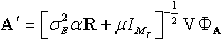 | (27) |
 | (28) |
 And,
And, 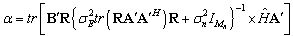 | (29) |
 | (30) |
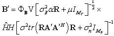
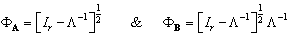
 are defined by the eigenvalue decomposition. V is the
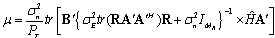
  matrix composed of the eigenvectors corresponding to non-zero eigenvalues. By putting (27) and (28) into (29) and (30) respectively, μ and α unknowns can be formulated in two equations which can be easily calculated.With increased number of iterations, the algorithm give the
  and
and  upto a unitary transform and a unique optimum covariance matrix can be obtained using
  .This optimum covariance matrix reduces to the capacity results as obtained in[4] if the estimated variance has been considered as zero. With the partial CSR knowledge, the optimum transmitters for maximized (7) and minimized (23) share the same structure differing only in power allocation. Finally, it has been seen that the optimum solution for (23) as
  and
and  gives the optimum solution for (7) using
  which further shows the global maximum for (7) and global minimum for (23).
 6. Results and Discussion
- The broad capacity analysis has been performed by deriving the order statics techniques, reducing the MSE, maximizing the mutual information by implementing the proposed algorithm followed by the improved results in enhancement of overall capacity and reduction in pilot symbols for different combination of MIMO antennas. Figure 3 shows the capacity of the different MIMO antenna combinations and their capacity increase with the increase in transmitting and receiving antenna elements for the condition when CSI is known to transmitter with the spatial heterogeneous behavior. It is clearly apparent from the existing analysis and simulated results that the capacity increases with the increase in transmitter and receiver antenna elements. It is known that with CSI, zero forcing beamforming completely removes the interference between the transmitting antenna in
 | (31) |
 | (32) |
 and large number of antennas, (32) can be determined. Figure 3 shows that the capacity increases with the increase in number of antennas K. With partial CSI,
  , the interference remain in the reception of the signals at the receiver end due to which denominator in (31) exists. Using[34], the capacity reduces to
  | (33) |
 denotes a distributed random variable with parameter (1, M+N-1). Figure 3 and Figure 4 shows the capacity for the partial CSI condition for 2x2 and 4x4 antenna configurations which shows that with lower SNR conditions, significant improvement in capacity has been seen with the increase in number of Antenna elements. Whereas in case when the SNR is high, capacity of MIMO system with spatial channel becomes interference limited which increase with the quantization factor B. Figure 3 shows that the capacity of the MIMO system with known CSI is better than the capacities with partial CSI or unknown CSI which has been limited due to lower bound conditions. Figure 4 shows the comparison of capacity with partial CSI and the new capacity found using adaptive method with partial CSI, which shows improvements at the lower SNR conditions as compared with the capacity with the partial CSI. At higher SNR conditions, this estimation scheme has also the interference limited bound with them but still a good result has been found using this estimation scheme as compared with the existing partial CSI condition, which has been achieved using the following bounds,
 | (34) |
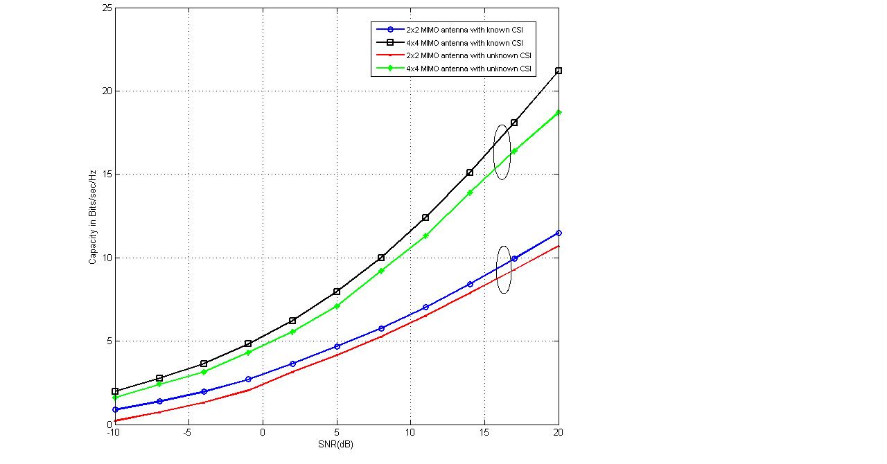 | Figure 3. Comparison of Capacity analysis for 2x2 and 4x4 MIMO antenna with known CSI and unknown CSI |
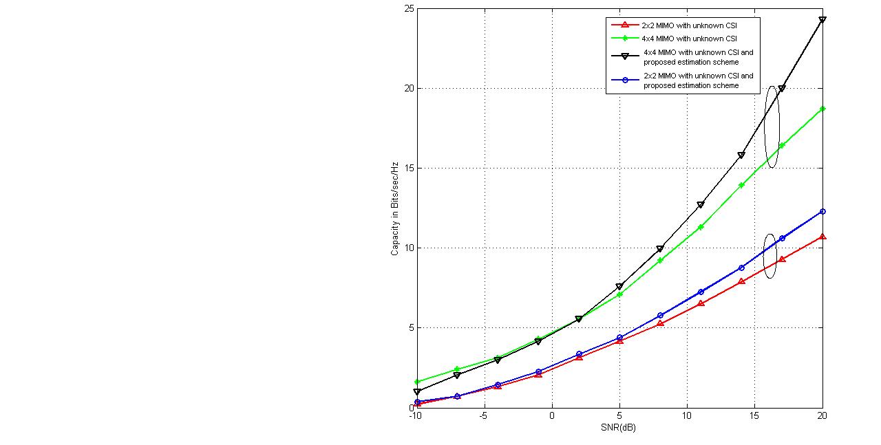 | Figure 4. Comparison of capacity analysis with unknown CSI for 2x2 and 4x4MIMO antenna for existing and proposed estimation scheme |
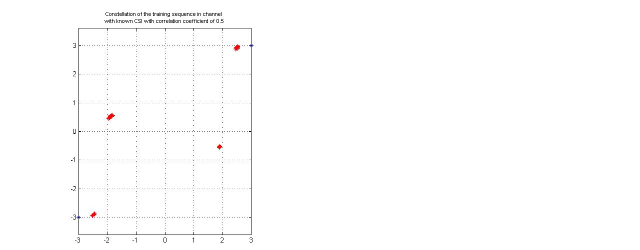 | Figure 5. Received training sequence constellation in channel with known CSI with correlation coefficient of 0.5 |
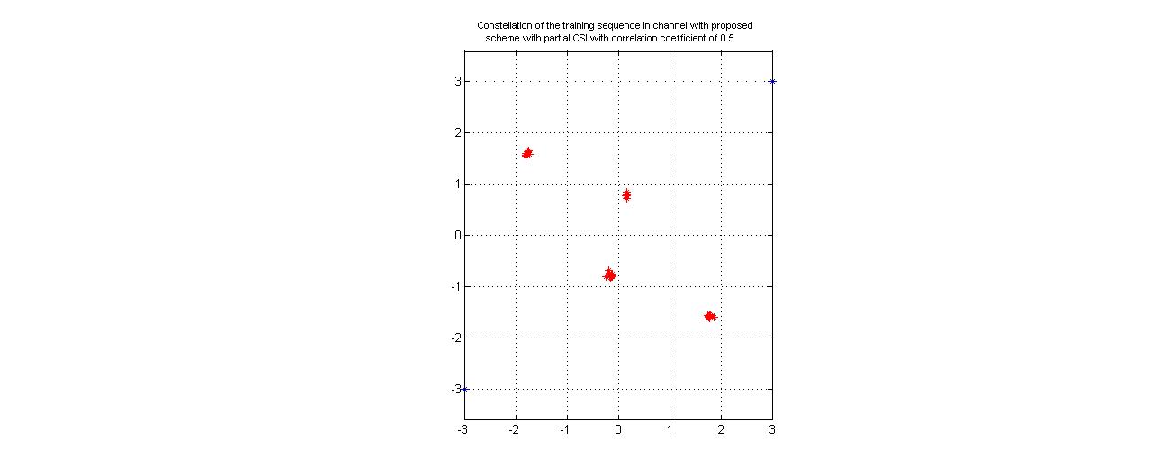 | Figure 6. Received training sequence constellation for channel with partial CSI with proposed estimation scheme with correlation coefficient of 0.5 |
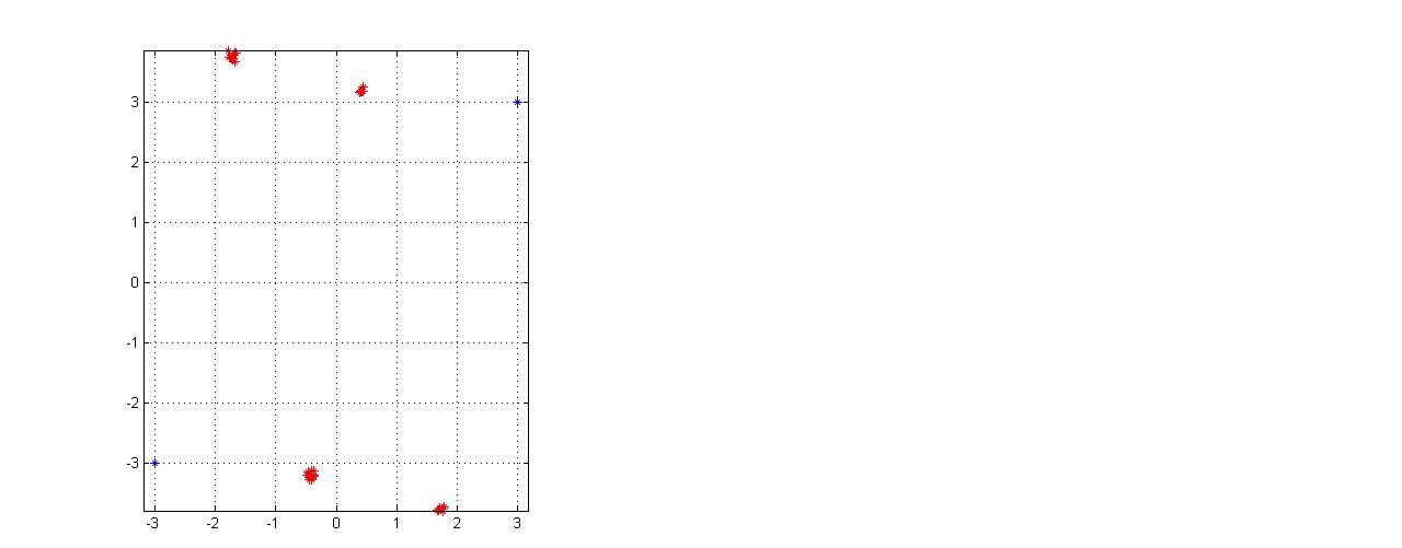 | Figure 7. Training sequence analysis for SNR 35dB with correlation coefficient of 0.5 for channel with partial CSI |
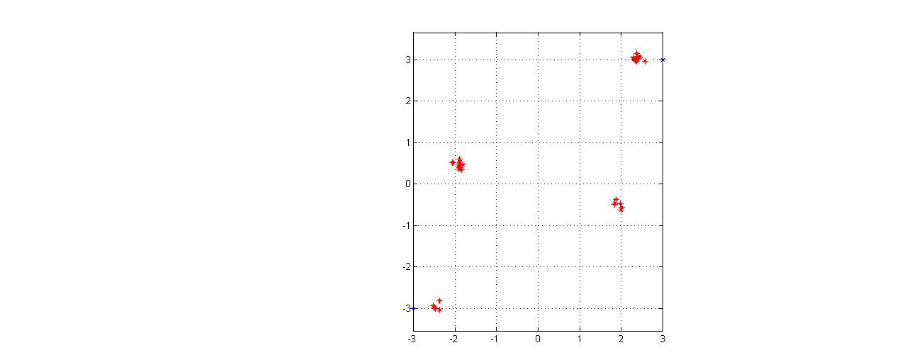 | Figure 8. Training sequence analysis for SNR 35dB with correlation coefficient of 0.5 for channel with partial CSI with proposed estimation scheme |
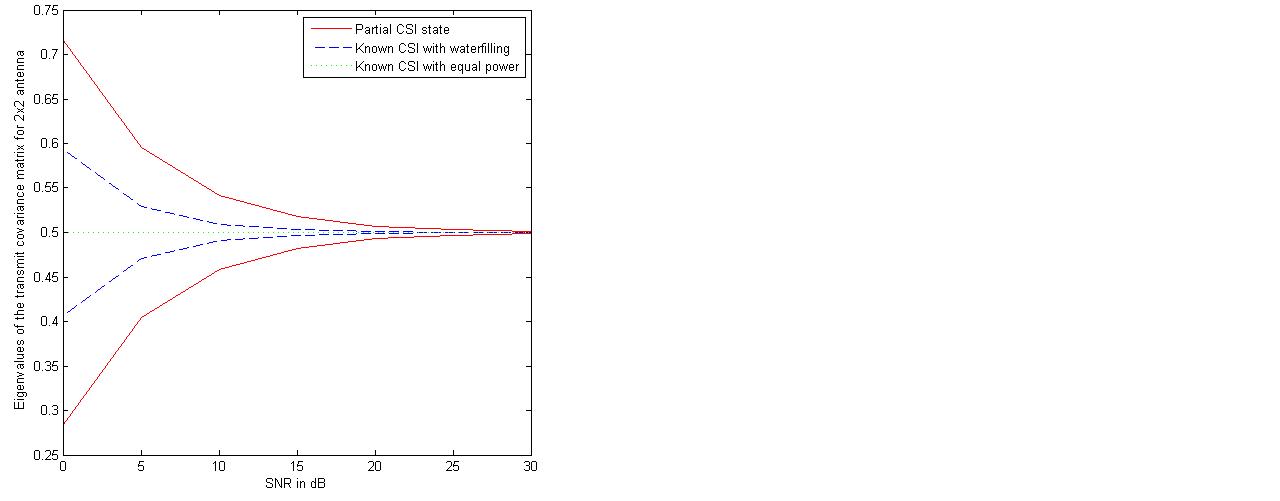 | Figure 9. Analysis of the eigenvalues of the transmit covariance matrix for 2x2 MIMO Antenna system |
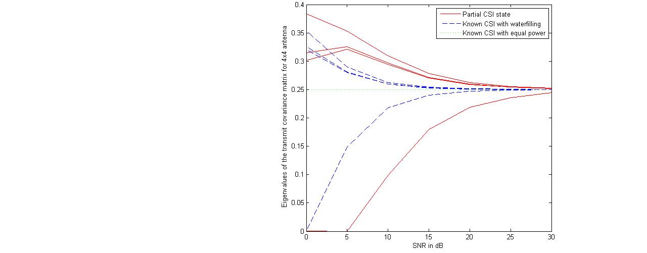 | Figure 10. Analysis of the eigenvalues of the transmit covariance matrix for 4x4 MIMO Antenna system |
7. Conclusions
- Design of a new adaptive algorithm has been proposed which has been implemented with the MIMO capacity lower bounds to maximize the capacity with the lower pilot symbols requirement in the partial CSI knowledge conditions for the spatial channels. Also the increase in mutual information and reduction in MSE has been tried with determination of optimum covariance matrix in precoder form for the transmit correlation matrix. The adaptive estimation based optimized precoded MIMO system shows the advantages in capacity enhancement as compared to the existing partial CSI conditions and equal power allocation scheme. Different estimation methods and comparison for transmitted training symbols have been tried and their improved results based on adaptive estimation method have been shown with the consideration of different correlation coefficient values for the transmitting antennas. Finally, the optimized capacity achieving eigenvalues of the transmit covariance matrix has been shown which is based on the eigenvectors knowledge of transmit covariance matrix, and found that the gap between the power of eigenvectors for higher antenna configurations has been reduced and it started to follow the equi-power channel mutual information.
ACKNOWLEDGEMENTS
- The author thankfully acknowledges the support provided by the authorities of Jaypee University of Engineering and Technology, Guna, India.