-
Paper Information
- Paper Submission
-
Journal Information
- About This Journal
- Editorial Board
- Current Issue
- Archive
- Author Guidelines
- Contact Us
Journal of Nuclear and Particle Physics
p-ISSN: 2167-6895 e-ISSN: 2167-6909
2019; 9(2): 59-68
doi:10.5923/j.jnpp.20190902.03

Quantum Theory of Circuit Systems – I. Aspects of Symmetry Principles and a Generalization of the Nonlinear Schrödinger Equation in Charge Space
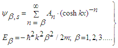
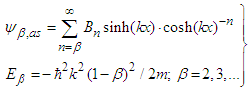
 Abstract
 Reference
 Full-Text PDF
 Full-text HTML
W. Ulmer
Gesellschaft Qualitätssicherung in der Medizin, 73779 Deizisau and MPI of Physics, Göttingen, Germany
Correspondence to: W. Ulmer, Gesellschaft Qualitätssicherung in der Medizin, 73779 Deizisau and MPI of Physics, Göttingen, Germany.
| Email: |  |
Copyright © 2019 The Author(s). Published by Scientific & Academic Publishing.
This work is licensed under the Creative Commons Attribution International License (CC BY).
http://creativecommons.org/licenses/by/4.0/

The quantization of circuits finds many interesting applications, e.g. quantum computer, molecular and biophysics. The method can be extended to nuclear physics, if the exchange interactions between nuclear particles are described by currents. A system of mutually coupled circuits can be treated by the linear Schrödinger equation yielding symmetries such as SU2, SU3, SU4, etc. A generalization of the principles to a nonlinear/nonlocal Schrödinger is presented; the nonlocal exchange between elementary particles is mediated by a Gaussian kernel (integral transform) in the charge space. The SU3 (or SU4, if four charges Q1,…,Q4 are accounted for) are used as the basic structure of the circuits. In nonlocal fields these symmetries hold, in the same fashion, too, but the energy levels are not equidistant as it the case at circuit quantization, equivalent to the 3D harmonic oscillator. The Gaussian kernel assumes zero value in the positive half-plane with E > 0. To avoid this hindrance a kernel is proposed, which only uses terms up to the second order of the Gaussian kernel, and a self-interacting 3D oscillator keeps excitations of arbitrary order to indemnify the confinement of quarks.
Keywords: Linear/nonlinear Schrödinger equation, Quantization of circuits, Charge space, Symmetry principles
Cite this paper: W. Ulmer, Quantum Theory of Circuit Systems – I. Aspects of Symmetry Principles and a Generalization of the Nonlinear Schrödinger Equation in Charge Space, Journal of Nuclear and Particle Physics, Vol. 9 No. 2, 2019, pp. 59-68. doi: 10.5923/j.jnpp.20190902.03.
Article Outline
1. Introduction
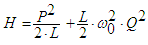
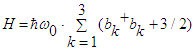
- The past decades have emerged novel application fields of quantum mechanics, namely the quantization of electromagnetic circuits. Thus an essential goal of these developments is the novel access to problems of radiation-, molecular- and biophysics. In particular, we mention the so-called 'Qubit' properties considered in molecular electronic devices, which make the requests the quantum computer feasible [1-10]. It although should be remembered that the first study to tread π-electrons of aromatic molecules by electric circuits now appeared about 70 years ago [11]. The basic principles of the quantization procedure are rather easily founded and well-known from textbooks in physics. Thus the Lagrangian
 of such a single oscillator reads:
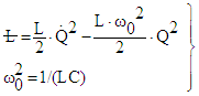 | (1) |
 | (2) |
 | (3) |
 | (4) |
 | (5) |
 | (6) |
 | (7) |
 | (8) |
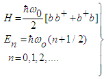
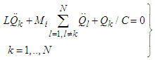
2. Systems of Coupled Circuits and the Generalization to a Nonlinear Schrödinger Equation in the Charge Space
2.1. Coupled Oscillators and Symmetry Properties
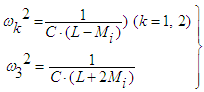
- Figure 1 shows a layer with 3 mutually coupled oscillators with magnetic coupling Mi. In a formal way we are able to write systems of N oscillators:
 | (9) |
 | Figure 1. 3 coupled oscillators with mutually magnetic interaction |
 | (10) |
 | (11) |
 | (12) |
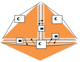
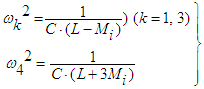
 | (13) |
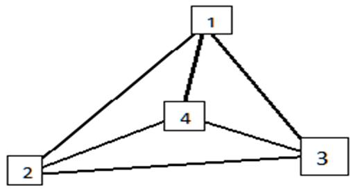 | Figure 2. 4 mutually coupled oscillators can be schematically shown by a tetrahedron |
 | (14) |
 | (15) |
 | (16) |
 | (17) |
2.2. Extension to the Nonlinear Schrödinger Equation (NSE)
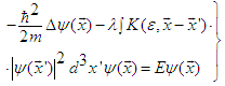
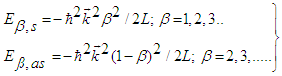
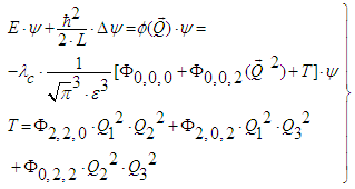
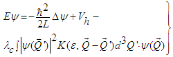
- The problem arises that neither with mechanical nor electric oscillators the energy differences between the energy levels remain constant. This fact is valid for atomic and molecular physics [16 - 18] as well as in nuclear physics. In similar fashion as with regard to a nonlinear, nonlocal Schrödinger equation containing a Gaussian kernel in the position space to account for the nonlocal influence (NNSE) we shall now pass to an outstanding generalization of the Schrödinger equation in the charge space. According to previous investigations the 3D version of the NNSE reads [18,19]:
 | (18) |
 | (19) |
 | (20) |
 | (21) |
 | (22) |
 | (23) |
 | (24) |
 | (25) |
 | (26) |
2.2.1. Some Properties of the Gaussian Kernel
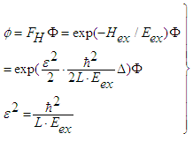
- Since the main interest is the charge space, we shall now study the nonlinear Schrödinger equation (NSE) and the nonlocal/nonlinear Schrödinger equation (NNSE) within this frame-work, the starting-point is an exchange Hamiltonian. The preceding aspects of convolution in the position space shall now be extended to the charge space, and we recall that the present considerations are valid in many different disciplines. Let
 be a distribution function and
  a source function, mutually connected by the operator FH; this represents an operator notation of a canonical ensemble. An exchange Hamiltonian Hex couples the source field Φ with an environmental field φ by FH, due to the interaction with surrounding charges. The partition function of a canonical ensemble reads:
 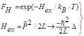 | (27) |
 | (28) |
 | (29) |
 | (29a) |
 | (30) |
 | (31) |
 | (32) |
 | (33) |
2.2.2. Nonlinear Schrödinger Equation in Charge Space with Local Interaction
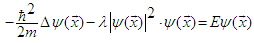
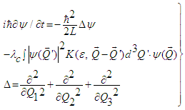
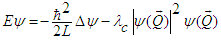
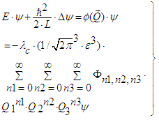
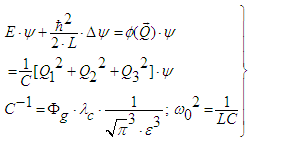
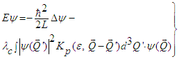
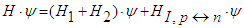
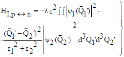
- In the sense of quantum electrodynamics (QED) is appears quite natural to take the self-interaction of charges into account. In the following, we only consider 3 different charges Q1, Q2, Q3. Since only the NNSE removes the property of equidistant energy levels, and we make use of this analogy and postulate a NNSE in charge space:
 | (34) |
 | (35) |
 | (36) |
2.2.3. Nonlinear/Nonlocal Schrödinger Equation in Charge Space (NNSE)
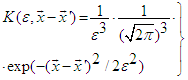
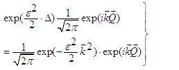
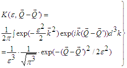
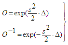
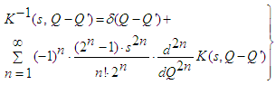
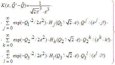
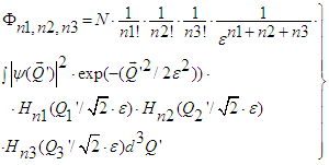
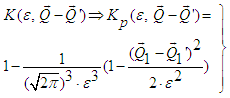
- With regard to the kernel K appearing in eq. (34) it is interesting to consider its generating function:
 | (37) |
 | (38) |
 | (39) |
 | (40) |
 | (41) |
 | (42) |
 | (43) |
 | (44) |
 | (45) |
 | (46) |
3. Results
3.1. Proton – Neutron – Deuteron Based on Quantized Circuits
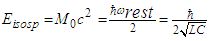
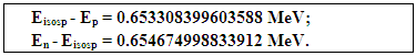
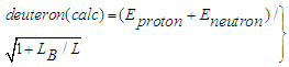
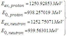
- The starting-point for p and n is the representation both particles as resonators and the assumption of two identical particles with only different iso-spin, i.e. their rest-energy amounts to:
 | (47) |
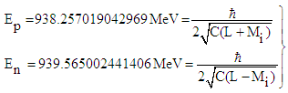 | (48) |
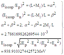 | (49) |
 The deuterium model based on resonators is shown by Figure 3. The principal coupling Mi between the resonators corresponds to eqs. (47 - 49). There are two additional branches referring to the motion of p and n denoted by LM, which are connected to the capacitances. In order to determine the normal modes we consider the equations according to eq. (49) and the succeeding equations (50) and (51):
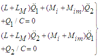 | (50) |
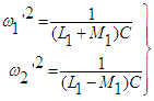 | (51) |
 | (51a) |
 | (51b) |
 In Figure 3 the motion of the proton and neutron is denoted by currents with LM and mutual coupling between protons – neutrons by Mim. The aspect of iso-spin and spin did not play a decisive role in the above considerations. At first we point out that eq. (47) is immediately related to iso-spin, i.e. we have two identical nucleons differing in the related quantum number.
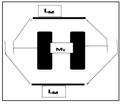 | Figure 3. Deuteron model with the constituents p and n |
 | (52) |
 | (52a) |
3.2. Proton – Neutron – Deuteron via NNSE in Charge Space
3.2.1. Proton - Neutron
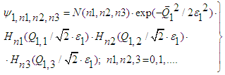
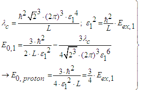
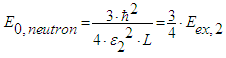
- It should be mentioned that the proton quarks are given by [(2/3)e0, (2/3)e0, - (1/3)e0] and the neutron quarks by [[(2/3)e0,-1/3)e0, -(1/3)e0], the square of proton quarks yields the effective charge 2∙(4/9)∙e02 + (1/9)∙e02 = e02, whereas for the neutron we obtain (4/9)∙e02 + 2∙(1/9)∙e02 = (2/3)∙e02. This fact is important with regard to the normalization.With respect to the following equations we use the nomenclature: the bold ‘1’ refers to proton index and the neutron index is characterized by ‘2’. As already previously point out the basic equation for protons (and neutrons) is given by the following equation:
 | (53) |
 | (54) |
 | (55) |
 | (56) |
 | (57) |
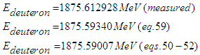
3.2.2. Deuteron
- The basic equation reads:
 | (58) |
 | (59) |
4. Conclusions
- With regard to deuteron we should like to point out that we could not verify of an excited overall state, although the proton/neutron quarks may undergo excitations. By that, excited resonance states are obtained, which are well-known in particle physics. In last time, some debate arose, whether deuterons have excited states, but we are unable to confirm these speculations [23].It should further be pointed out that in a continuation we consider a nonlinear Dirac equation with self-interaction based on [10]. By that, we shall obtain a rather interesting form of Quantum Chromo-Dynamics (QCD) formulated by quantization of the charge space.