1. Introduction

The application of the Bethe-Bloch equation (BBE) for the determination of the electronic stopping power is established for the passage of electrons and protons through homogeneous media. A particular importance of BBE appears in Monte-Carlo calculations to simulate the behaviour (energy transfer) of charged projectile particles along the track. This equation reads:

(1)

E_I is the atomic ionization energy, weighted over all possible transition probabilities of atomic/molecular shells, and q denotes the charge number of the projectile (proton: q = 1, carbon: q = 6). The meaning of the correction terms a_shell, a_Barkas, a₀ and a_Bloch are explained in literature[1 – 6]. Since the Bloch correction a_Bloch will be introduced in equation (12), we present, for completeness, the remaining correction terms according to ICRU49[4]:

(2)

(3)

(4)

Some comments to the relations (2 – 4):

The parameter C, referring to shell corrections, is determined by different models ([4, and references therein]). A unique parameterization of C depending on Z, A_N, and E_I does not exist. It is therefore recommended to select C according to proper domains of validity. It must be noted that several models have been proposed to account for shell transitions. Therefore, the recommendations in[4] have been applied in this work.

The function F_ARB in equation (4) refers to the theory of the Barkas effect developed in[7]. The parameter α refers to Sommerfeld’s fine structure constant and b to a fitting parameter. Unfortunately, b is not a unique fitting parameter; this results in an uncertainty of about 2 %. Modifications of this equation with regard to high-Z materials are not of interest in this work. The Barkas effect represents a correction of BBE due to the electron capture of the positively charged protons at lower energies in the domain of the Bragg peak and behind leading to a slightly increased range R_csda, whereas the negatively charged anti-protons cannot capture electrons from the environmental electrons. Therefore their range is slightly smaller. With regard to protons this kind of correction works, i.e. the charge q² = 1 is assumed along the total proton track. For charged ions such as He or C⁶ it appears to be insufficient to keep the nuclear charge constant along the total track and to restrict the electron capture only to the small Barkas correction[8]. This means that all positively charged projectile particles stand in permanent exchange of energy E and charge q with environment, and, as a consequence, q² is a function of the actual residual energy, i.e. q² = q²(E), and only for E = E₀ (initial energy) q² = q₀² is valid. A correct modification of BBE by accounting for q²(E) makes the Barkas correction superfluous.

A further critical aspect of BBE, which leads to a modification by accounting for q²(E), is the range R_csda (csda: continuous slowing down approximation) of the electronic stopping power. Thus a naive application of BBE would lead to the conclusion that a carbon ion requires the initial energy per nucleon E₀ (carbon ion) = 3 times E₀(proton), since the square of the carbon charge amounts to 36 and the nuclear mass unit is 12 times nuclear mass unit of the proton. However, the ratio is not 3 to obtain the same range R_csda, but about 25/12. The Monte-Carlo code GEANT4 assumes an average charge q_Average = 5.06 for the simulations of the carbon tracks. This is, however, not satisfactory, since electron capture is a dynamical process. Therefore the range of charged particles has been subjected to many studies due to the increasing importance of carbon ions in radiotherapy[9–24].

It is also possible to substitute the electron mass m by the reduced mass m μ = m/(1+m/M), where M is the proton mass. However, this leads for protons to a rather small correction (i.e., less than 0.1 % for protons). For complex systems E_I and some other contributions like a_shell and a_Barkas can only be approximately calculated by simple quantum-mechanical models (e.g., harmonic oscillator); the latter terms are often omitted and E_I is treated as a fitting parameter, but different values are proposed and used[4]. The restriction to the logarithmic term leads to severe problems, if either v → 0 or 2m v² /E_I → 1. It should be added that a correct treatment of the electron capture removes the singularity of positively charged ions, since q²(E) → 0, if the residual energy E assumes zero.

2. Methods

2.1. The Integration of BBE for Protons

In the following, we consider at first the integration of BBE for protons, i.e. we consider the Barkas correction in the conventional way. In previous publications[25–26] we have presented an analytical integration of BBE, which is the physical base of the transport of protons and electrons.

In order to obtain the integration of BBE, we start with the logarithmic term and perform the substitutions:

(5)

With the help of substitution (and without any correction terms), BBE leads to the integration:

(6)

The boundary conditions of the integral are:

(7)

The general solution is given by the Euler exponential integral function Ei(ξ) with P.V. = principal value:

(8)

Some details of Ei(ξ) and its power expansions can be found in[27]. The critical case ξ = 0 results from E_critical = ME_I/4m (for water with E_I = 75.1 eV, the critical energy E_critical amounts to 34.474 keV; for Pb with E_I ≈ 800 eV to about 0.4 MeV). Since the logarithmic term derived by Bethe implies the Born approximation, valid only if the transferred energy E_transfer >> the energy of shell transitions, the above corrections, excepting the Bloch correction, play a significant role in the environment of the Bragg peak, and the terms a₀ and a_shell remove the singularity. With respect to numerical integrations (Monte Carlo), we note that, in the environment of E = E_critical, the logarithmic term may become crucial (leading to overflows); rigorous cutoffs circumvent the problem. Therefore, the shell correction is an important feature for low proton energies. In similar fashion, we can take account of the Barkas correction. Since this correction is also important for low proton energies, it is difficult to make a quantitative distinction to the shell correction, and different models exist in the literature implying overall errors up to 2 %[4]. Using the definitions/suggestions of the correction terms according to[4] and the substitutions we obtain:

Some details of Ei(ξ) and its power expansions can be found in[27]. The critical case ξ = 0 results from E_critical = ME_I/4m (for water with E_I = 75.1 eV, the critical energy E_critical amounts to 34.474 keV; for Pb with E_I ≈ 800 eV to about 0.4 MeV). Since the logarithmic term derived by Bethe implies the Born approximation, valid only if the transfer energy E_transfer >> the energy of shell transitions, the above corrections, excepting the Bloch correction, play a significant role in the environment of the Bragg peak, and the terms a₀ and a_shell remove the singularity. Therefore, the shell correction is an important feature for low proton energies. In similar fashion, we can take account of the Barkas correction. Since this correction is also important for low proton energies, it is difficult to make a quantitative distinction to the shell correction, and different models exist in the literature implying overall errors up to 2 %[4]. Using the definitions/suggestions of the correction terms according to[4] and the substitutions we obtain:

(9)

A closed integration of equation (9) does not exist; it can be evaluated via a procedure valid for integral operators[28], which reads for commutative operators:

(10)

A’+B’ is equated to the complete denominator on the right-hand side of equation (9).The small Barkas correction and the Bloch correction a_Bloch (see equations 12, 13) are identified with A’ and the other (more important) terms with B’:

(11)

We should already point out here that the expansion (10) is also applicable, if the electron capture is accounted for. The integration of equation with the help of relation (10) leads to standard tasks (i.e. to a series of usual exponential functions). In the following, we add the Bloch correction to the denominator of equation. In order to use the procedure, we define now the non-relativistic energy E_nr by: E_nr = 0.5∙Mv² and write the relativistic energy expression E_rel (the rest energy Mc² is omitted) in terms of an expansion:

(12)

Relation (12) provides a sequence of exponential functions:

(13)

(14)

The integration of equation is carried out with the boundary conditions. Since these conditions are defined by logarithmic values, which have to be inserted to an exponential function series, the result yields a power expansion for R_CSDA in terms of E₀:

(15)

The coefficients α_n are determined by the integration procedure and only depend on the parameters of the BBE. For applications to therapeutic protons, i.e., E₀ < 300 MeV, a restriction to N = 4 provides excellent results (Figure 1). For water, we have to take E_I = 75.1 eV, Z/A_N = 10/18, ρ = 1 g/cm³; Formula (15) becomes:

(16)

The values of the parameters of Formulas with restriction to N = 4 are displayed in Tables 1 and 2.

Table 1. Parameter values for equation (15), E0 in MeV, EI in eV and RCSDA in cm α1 α2 α3 α4 6.8469∙10-4 2.26769∙10-4 -2.4610∙10-7 1.4275∙10-10 p1 p2 p3 p4 0.4002 0.1594 0.2326 0.3264

The determination of A_N and Z is not a problem in case of atoms or molecules, where weight factors can be introduced according to the Bragg rule; for tissue heterogeneities, it is already a difficult task. Much more difficult is the accurate determination of E_I, which results from transition probabilities of all atomic/molecular states to the continuum (δ- electrons). Thus with regard to stopping powers of protons in different media according to[4], there are sometimes different values of E_I proposed (e.g., for Pb: E_I = 820 eV and E_I = 779 eV). If we use the average (i.e., E_I = 800.5 eV), the above formula provides a mean standard deviation of 0.27 % referred to stopping-power data in[4], whereas for E_I = 820 eV or E_I = 779 eV we obtain 0.35 % - 0.4 %. If we apply the above formula to data of other elements listed in[4], the mean standard deviations also amount to about 0.2 % - 0.4 %.

Table 2. Parameter values for equation (16), E0 in MeV, EI in eV and RCSDA in cm a1 a2 a3 a4 6.94656∙10-3 8.13116∙10-4 -1.21068∙10-6 1.053∙10-9

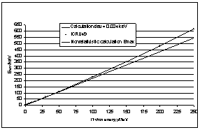
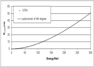
Figure 1. Comparison data in[4] of proton RCSDA range (up to 300 MeV) in water and the fourth-degree polynomial (equation 16). The average deviation amounts to 0.0013 MeV

Instead of the usual power expansion (16), we can represent all integrals in terms of Gompertz-type functions multiplied with a single exponential function by collection of all exponential functions obtained by the expression of[A’ +B’]^-1 and the substitution . A Gompertz- function is defined by:

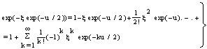
(17)

By the integration boundaries u = 2∙ln∙4m∙E₀/(M∙E_I), i.e., E = E₀ and u → ∞ (E = 0), the integration leads to a sequence of exponential functions; the power expansion is replaced by:

(17a)

For therapeutic protons, the restriction to N = 2 provides the same accuracy (Figure 2) as formula (16); the parameters are given in Table 3 (a₁ is the same as in Table 2).

Table 3. Parameters of Formula (17a); b1 and b2 are dimensionless; g1 and g2 are given in MeV-1. b1 b2 g1 g2 15.14450027 29.84400076 0.001260021 0.003260031

In the following, we shall verify that the latter formula provides some advantages with respect to the inversion E₀ = E₀(R_CSDA).

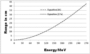
Figure 2. RCSDA calculation - comparison between a fourth-degree polynomial (equation (16)) and two exponential functions (equation (17a))

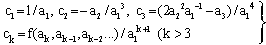
2.2. The Inversion Problem: Calculation of E₀(R_CSDA) and E(z)

Above formulas can also be used for the calculation of the residual distance R_CSDA – z, relating to the residual energy E(z); we have only to perform the substitutions R_CSDA → R_CSDA – z and E₀ → E(z) in these formulas. In various problems, the determination of E₀ or E(z) as a function of R_CSDA or R_CSDA – z is an essential task. The power expansion implies again a corresponding series E₀ = E₀(R_CSDA) in terms of powers:

(18)

(18a)

The coefficients c_k are calculated by a recursive procedure; we have given the first three terms in formula (18a). Due to the small value of a₁ = 6.8469∙10^-4, this series is ill-posed, since there is no possibility to break off the expansion; it is divergent and the signs of the coefficients c_k are alternating, see[27]. The inversion procedure of equation leads to the formula:

(19)

The inverse formula of equation (17a) reads:

(20)

For therapeutic protons, a very high precision is obtained by the restriction to N = 5 (Table 4 and Figure 3). Formula (20) is also suggested by the consideration of S(R_CSDA) = E₀(R_CSDA)/R_CSDA according to equation (17a). A plot of S(R_CSDA) has been previously presented[25]; it gives rise for an expansion of S(R_CSDA) in terms of exponential functions.

Table 4. Parameters of the inversion Formula (40) with N = 5 (dimension of ck: cm/MeV, λk: cm-1) P1 P2 P3 P4 P5 -0.1619 -0.0482 -0.0778 0.0847 -0.0221 q1 q2 q3 q4 q5 0.4525 0.195 0.2125 0.06 0.0892 c1 c2 c3 c4 c5 96.63872 25.0472 8.80745 4.19001 9.2732 λ1-1 λ2-1 λ3-1 λ4-1 λ5-1 0.0975 1.24999 5.7001 10.6501 106.72784

One way to obtain the inversion formula is to find S(R_CSDA) by a sum of exponential functions with the help of a fitting procedure. Thus it turned out that the restriction to five exponential functions is absolutely sufficient and yields a very high accuracy. A more rigorous way (mathematically) has been described in the LR of[25].

The residual energy E(z), appearing in equation (20), is the desired analytical base for all calculations of stopping power and comparisons with GEANT4. The stopping power is determined by dE(z)/dz and yields the following expression:

(21)

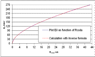
Figure 3. Test of the inverse Formula (40) E0 = E0(RCSDA) by five exponential functions. The mean deviation amounts to 0.11 MeV; the plot results from Figure 1

The aforementioned restriction to N = 5 is certainly extended to equation (21), which can be considered as a representation of the BBE in terms of the residual energy E(z). Due to the low-energy corrections (a₀, a_shell, a_Barkas) the energy-transfer function dE(z)/dz remains finite for all z (i.e., 0 ≤ z ≤ R_CSDA). This is, for instance, not true for the corresponding results at z = R_CSDA. The calculation of E(z) and dE/dz according to equations, referred to as LET, is presented in Figure 4. The figure shows that, within the framework of CSDA, the LET of protons is rather small, except at the distal end of the proton track.

A change from the interacting reference medium water to any other medium can be carried out by the calculation of R_CSDA, where the substitutions have to be performed:

(22)

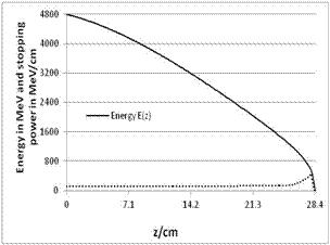
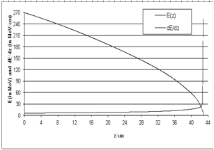
Figure 4. E(z) and dE(z)/dz as a function of z (LET based on CSDA); energy straggling and electron capture are omitted

It is also possible to apply formula (22) in a stepwise manner (e.g., voxels of CT). This procedure will not be discussed here, since it requires a correspondence between (Z∙ρ/A_N)_Medium and information provided by CT. The application of BBE is a more difficult task with regard to heterogeneous media based only on CT data.

2.3. Qualitative Properties of the Electron Transfer Described by BBE and Electron Capture

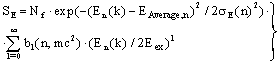
According to BBE the energy spectrum produced by carbon ions should be the same as that produced by protons, and the only difference between protons and carbon ions should be the intensity of the released collision electrons, i.e. the amplification factor should be 36 for carbon ions. It is well-known that this property is not valid for the following reasons: The average ionization energy for carbon ions turned out to be E_I = 80 eV instead of E_I = 75 eV for protons[4, 29]. Paper[29] is based on investigations of some other authors[10, 19, 30, 31]. The second reason is the electron capture of the carbon ion. Thus a carbon ion can capture a free electron, which has been excited immediately before. Figure 5 shows this effect. However, only electrons with a slow relative velocity to the carbon ion can account for this process (v_relative ≈ 0). Since the transition time of the capture electron to a lower atomic state of the carbon ion is less than 10^-10 sec with a simultaneous emission of light (UV or visible), it is possible that the captured electrons goes lost again, and only a stripping effect occurs for a short time. If the C⁶⁺ ions has been finally transferred to a stable C⁵⁺ ion, the identical process can be repeated until at the end track a neutral carbon atom is obtained having only a thermal energy. In the environment of the Bragg peak the effective charge of the carbon ion is about the same that of a proton, namely +e₀. Since the electron capture can only occur for electrons of which the relative velocity is slow, the upper energy limit of the energy exchange E_ex is the Fermi edge E_F, which is for an electron gas not higher than the thermal energy k_BT. If the charge of carbon ion amounts to +6·e₀ and, at least, > +e₀, the environmental atomic electrons suffer lowering of the energy levels due to the Coulomb interaction, which leads to an increase of E_I. Therefore the stated value of E_I = 80 eV represents an average value produced the fast carbon ion starting with +6·e₀ and ending with an uncharged, neutral carbon atom.

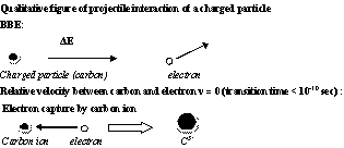
Figure 5. Excitation of an atomic electron by the collision interaction of a fast carbon ion with an atomic electron and the reversal process of the electron capture

2.4. Application Fermi-Dirac Statistics to Electron Capture

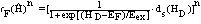
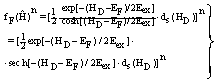
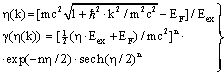
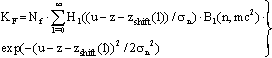
In the following it is the task to obtain a quantum statistical description of electron capture and stripping of electrons, i.e. those electrons which reduce the effective charge of the carbon ion for a short time and go lost before a transition to a stable atomic state of carbon can occur. For this purpose, we consider the quantum statistical energy exchange E_ex between projectile particle such as proton, He ion or carbon ion. The related mathematical procedure can be used to describe processes like energy straggling, lateral scatter and energy/charge exchange between projectile ion and released electrons below the Fermi edge E_F. However, before we can account for the latter problem we have to consider the related mathematical tools.

In general, if H represents the Hamiltonian (either non-relativistic or relativistic) and f(H) an operator functions, then for continuous operators H the connection holds:

(23)

At first we apply this relation in the non-relativistic case to derive the Gaussian convolution for the description of energy straggling. If the stopping power S(z) = dE(z)/dz of protons is calculated by BBE or by phenomenological equations (13, 22) based on classical energy dissipation, then the energy fluctuations are usually accounted for by:

(24)

This kernel may either be established by non-relativistic transport theory (Boltzmann equation) or, as we prefer here, by a quantum statistical derivation. Let φ be a distribution function and Φ a source function, mutually connected by the operator F_H (operator notation of a canonical ensemble):

(25)

An exchange Hamiltonian H couples the source field Φ (proton fluence) with an environmental field φ by F_H, due to the interaction with electrons:

(26)

It must be noted that the operator equation (26) was formally introduced[32] to obtain a Gaussian convolution as Green’s function and to derive the inverse convolution. F_H may formally be expanded in the same fashion as the usual exponential function exp(ξ); ξ may either be a real or complex number. This expansion is referred to as Lie series of an operator function. Only in the thermal limit (equilibrium), can we write E_ex = k_BT, where k_B is the Boltzmann constant and T is the temperature. This equation can be solved by the spectral theorem provided by the discipline ‘functional analysis’:

(27)

It is a noteworthy result[25] that a quantum stochastic partition function leads to a Gaussian kernel as a Green’s function, which results from a Boltzmann distribution function and a non-relativistic exchange Hamiltonian H. An operator formulation of a canonical ensemble is obtained by the following way: let φ be a distribution (or output/image) function and Φ a source function, which are mutually connected by the operator. In a 3D version, linear combinations of K(σ, u – x) and the inverse kernel K^-1 are also used in scatter problems of photons[32]. As an example, we consider the Schrödinger equation of a free electron transferring energy from the projectile to the environment and obeying a Boltzmann distribution function f(H) = exp(-H/E_ex):

(28)

The above relation provides:

(29)

In the case of thermal equilibrium, we can replace the exchange energy E_ex by k_BT.

With regard to our task the Dirac equation to describe the particle motion is an adequate starting-point:

(30)

Please note that in the notation of equation (30) refers to the Pauli spin matrices (this should not be confused with the rms-value σ of a Gaussian distribution function). In position representation we obtain:

(31)

According to[28] we can write:

(32)

E_Pauli is the related energy value resulting from the Pauli equation.

From the view-point of the many-particle-problem Fermi-Dirac statistics is adequate mean by the notation of operator functions:

(33)

E_F represents the energy of the Fermi edge (usually some eV) and d_s the density of states of the Hamiltonian H_D. The iterated operator function reads:

(34)

By that, the above expression assumes the shape:

(35)

In order to obtain a convolution kernel of a generalized Gaussian type by multiplication with Hermite polynomials, we make use of the following expansion[26]:

(36)

(37)

E_l (l = 0, 1, 2, …,) refer to Euler numbers[27].

The spectral theorem of functional analysis provides:

(38)

By performing all integrations we obtain:

(39)

In the position space equation (39) assumes the shape:

(39a)

According to Bohr’s formalism[1] the formula for energy straggling (or fluctuation) S_F is given by:

(40)

The fluctuation parameter σ_E can be best determined using the method in[1]. Furthermore we can verify the connection between E_Average in the theory of Bohr and the Fermi edge energy E_F, since E_Average results from the repeated iteration of E_F (for finite intervals of Δz):

(41)

Δσ_E² contains as a factor the important magnitude E_max, that is, the maximum energy transfer from the proton to an environmental electron; it is given by E_max = 2mv²/(1-β²). In a non-relativistic approach, we get E_max = 2mv². E_max can be represented in terms of the energy E, and, for the integrations to be performed, we recall the relation E = E(z) according to formula (40); the comparison to ICRU49 data is presented in Figure 6:

(42)

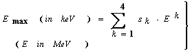
Figure 6. Calculation of Emax according to equation (42). The straight line below refers to the non-relativistic limit

Table 5. The parameters sk for the calculation of Emax (formula (42)) s1 s2 2.176519870758 0.001175000049 s3 s4 -0.000000045000 0.0000000000348

However, we should like to point out that according to the preceding section this determination is only valid for protons and cannot be applied to heavy ions without a change of the parameters. As in the previous section, we use the definition of S(z) according to BBE. S(z) is proportional to q²:

(44)

The application of equations (35 - 39) and the transition to the continuum provides (up to 2nd order):

(44a)

The R_CSDA formula (equation (16)) now becomes:

(45)

The parameters have slightly to be modified: α=0.00694650.0008132157, γ = - 0.00000121069, δ = 0.000000001051.

3. Results

In the following we present results of calculations for protons, He ions and carbon ions; the initial energy amounts to 400 MeV/nucleon. This appears to be a reasonable restriction with regard to therapeutic conditions. Thus Figure 7 shows that at the end of the projectile track all charged ions nearly behave in the same manner.

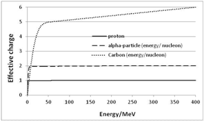
Figure 7. Effective charge of protons, He- and C-ions as a function of the initial energy E0 (for protons, we have to assume qeff = 0.995)

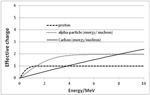
Figure 8. Section of the above Figure 7 for E ≤ 10 MeV

Figure 8 provides a more detailed behaviour in the low energy domain. The residual energy per nucleon amounts to 10 MeV or smaller.

Figure 9 presents for three cases the decrease of the actual charge of carbon ions in dependence of the initial energy E₀/nucleon. Thus we can conclude that for residual energies E < 50 MeV/nucleon the behaviour of the carbon ions does not depend on the initial energy E₀.

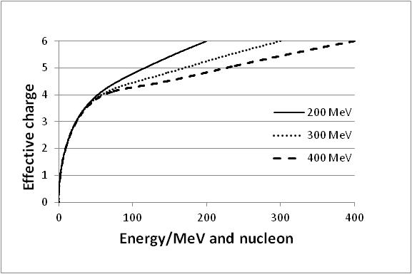
Figure 9. Effective charge q(E) of carbon ions in dependence of the initial energy E0 for the cases E0 = 200, 300 and 400 MeV/nucleon

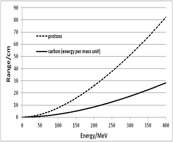
Figure 10. Comparison between proton range calculated by Formula (16) and range of the carbon ion determined by Formula (45)

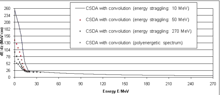
Figure 11. Stopping power of protons in dependence of the energy straggling (mono-energetic and polychromatic protons without taking account of electron capture)

Since Figure 10 is restricted to the energy per mass unit, it is apparent that an enormous amount of energy is required to accelerate carbon ions to therapeutic ranges. This is certainly one obstacle for the radiotherapy with carbon ions.

With regard to the therapeutic efficacy the behaviour of the LET in the environment of the Bragg peak is very significant. For a comparison, we first regard a previous result[26, 33] referring to the LET of protons. According to Figure 11 the stopping power of protons at the end track depends significantly on the initial energy E₀ and on the beam-line (energy spectrum at the impinging plane). The electron capture of the proton at the end track is ignored. However, the previous Figure 8 clearly shows that for protons the electron capture only becomes more significant, if the actual proton energy satisfies E < 2 MeV. The electron capture of protons at the end track would make the LET of protons zero independent of the initial energy.

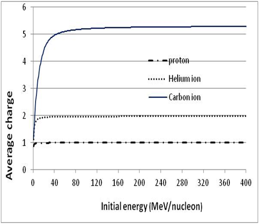
Figure 12. Average charge of protons, He and C ions as a function of the initial energy E0 (for protons, we have to assume qeff = 0.995)

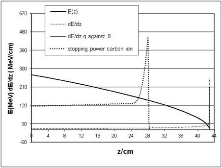
Figure 13. LET for mono-energetic protons (dots) and overall stopping power S(z) of carbon ions 400 MeV/nucleon

Figure 14. LET of carbon ions (400 MeV/nucleon)

Figure 12 is important with regard to Monte Carlo applications, since it determines the actual value of q_eff to be used in dependence of E₀. The succeeding Figure 13 presents E(z) and S(z) = dE(z)/dz of protons and S(z) of carbon ions by taking account for electron capture. The initial proton energy amounts to 270 MeV, whereas the initial carbon ion energy is 400 MeV/nucleon. Most significant is the height of the Bragg peak, which is resulting from the electron capture only a factor 1.7 higher than that of protons. In both cases the csda approach is assumed. Since protons are much more influenced by energy straggling and scatter, their peak height are reduced again, whereas for carbon ions scatter and energy straggling do not play a very significant role due to the mass factor 12.

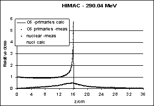
Figure 15. Measurement (HIMAC) and theoretical calculation of the Bragg curve of carbon ions (290 MeV/nucleon)

A rigorous consideration of the LET of carbon ions is given the following Figure 14. It makes only sense to consider the total energy of 4800 MeV of the carbon ions. Due to this order of magnitude E(z) of the carbon ion has not been presented in Figure 13. Energy straggling and scatter have been ignored in Figure 14, which is justified for heavy carbons. On the other side, this figure makes also apparent the well-known disadvantage of carbon ions, namely the enormous amount of energy of carbon ions in order to reach an acceptable dose distribution in the domain of the target, where a SOBP is required. With the help of GEANT4 a real depth dose curve (HIMAC, 290 MeV/nucleon[14–15]) has been determined. The role of GEANT4 was only to account for the nuclear reactions, which are based in this Monte-Carlo code on an evaporation model. The electronic stopping power S(z) has been determined by the tools worked out in this communication, the electron capture effect has been accounted for. Further parameters for a calculation of S(z) have been used based on the proton calculation model[26, 33] by appropriate modifications. The Gaussian convolution kernels for energy straggling and lateral scatter have been rescaled according to the corresponding mass properties.

With regard to the decrease of fluence of primary carbon ions we have derived some modifications of the corresponding decrease curves for protons. However, it appears not to be appropriate to go into further details. A further aspect is the use of the code GEANT4. Since this Monte- Carlo code represents an open programming package, some suitable additional reaction channels have been introduced with reference to nuclear reaction detected by HIMAC:

4. Conclusions

The main purpose of this communication was the derivation of a systematic theory of electron capture of charged particles and the role for the LET. The role of the LET of light ions with regard to the biological effectiveness has recently been studied[34]. There are purely empirical trials to include charge capture in Monte-Carlo codes[10 – 13, 35 – 36]. However, it appears that a profound basis for the calculation of q²(E), E(z), S(z) and R_csda(E₀) depending besides the initial energy E₀ also on the nuclear mass number N is required to account for further influences of Bragg curves such as the density of the medium and its nuclear mass/charge A_N and Z. The unmodified use of BBE leads to wrong results and the Barkas correction, which does not affect the factor q² of BBE, only works for protons or antiprotons, whereas for projectile particles like He or carbon ions this correction cannot be considered as small. The presented theory includes the Barkas effect without any correction model. In view of the enormous effort with reference to the acceleration of C⁶ ions, the application of this therapy modality should be critically reviewed.

ACKNOWLEDGEMENTS

The author wishes to thank Dr. Barbara Schaffner. Due to her sabbatical work at HIMAC, Japan, the analysis of Figure 15 has been made available.

References

[1]  Bethe H. A., Ashkin J. ‘‘Passage of radiations through matter’’ Experimental Nuclear Physics (E. Segrè Ed.) Wiley New York, 176 – 190, 1953.
[2]  Bloch F. ‘‘Zur Bremsung rasch bewegten Teilchen beim Durchgang durch Materie‘‘ Ann der Physik 16, 285 – 292, 1993.
[3]  Bethe H. A. ‘’Molière’s theory of multiple scattering’’ Phys. Rev. 89, 1256 - 1262, 1953.
[4]  ICRU ‘’Stopping powers and ranges for protons and α-particles’’ ICRU Report 49 (Bethesda, MD), 1993.
[5]  CERN-Report: Monte-Carlo code GEANT4 GEANT4-Documents, 2005. http//geant4.web.cern.ch/geant4/G4UsersDocuments/Overview/html.
[6]  Boon S. N. ‘’Dosimetry and quality control of scanning proton beams’’, PhD Thesis Rijks University Groningen, 1998.
[7]  Ashley J. C, Ritchie R. H., Brandt W. ‘’Document No. 021192‘’, (National Auxilliary Service, New York), 1974.
[8]  Barkas W.H., Dyer N.J., Heckmann H. H. ‘’Resolution of the Mass Anomaly’’ Phys. Rev. Letters 11, 26 – 29, 1963.
[9]  Betz H. D. ‘’Charge States and Charge-changing Cross Sections of Fast Heavy Ions Penetrating through Gaseous and Solid Media’’ Rev. Mod. Phys. 44, 465 – 85, 1972.
[10]  Dingfelder M., Hantke D., Inokute M., Paretzke H.G. ‘’A Monte-Carlo code for heavy charged ions‘’ Radiation Physics and Chemistry 53, 1 – 20, 1998.
[11]  Gudowska I., Sobolevsky N., Andreo P., Belkic D., Brahme A. ‘’Ion beam transport in tissue-like media using the Monte-Carlo code SHIELD-HIT’’ Phys. Med. Biol. 49, 1933 – 38, 2004.
[12]  Hollmark M., Uhrdin J., Belkic D., Gudowska I., Brahme A. ‘‘Influence of multiple scattering and energy loss straggling on the absorbed dose distributions of therapeutic light ion beams: 1. Analytical pencil beam model’’ Phys. Med. Biol..49, 3247 - 3067, 2004.
[13]  Hubert F., Bimbot R., Gaurin H. ‘’Range and stopping-power tables for 2.5 – 500 MeV/nucleon heavy ions in solids’’ Data Nucl. Data Tables 46, 1 – 213, 1990.
[14]  Kanai T., Kohno T., Minohara S., Sudou M., Takada E., Soga F., Kawachi K. Fukumura A. ‘’Dosimetry and measured differential W values of air heavy ions’’ Rad. Res. 135, 293 – 301, 1993.
[15]  Kusano Y., Kanai T., Yonai S., Komori M., Ikeda N., Tachikawa Y., Ito A. Uchida H. ‘’Field-size dependence of doses of therapeutic carbon beams’’ Med. Phys. 34, 4016 – 4022, 2007.
[16]  Mairani A. ‘’Nucleus-Nucleus Interaction Modeling and Applications in Ion Therapy Treatment Planning’’, PHD-Thesis, University of Pavia, 2007.
[17]  Matveev V. I., Sidorov D.B. ‘’Effective Stopping of Fast Heavy Highly Charged Structure Ions in Collisions with Complex Atoms’’ JETP Letters 84, 234 – 248, 2006.
[18]  Sigmund P. ‘’Charge dependent electronic stopping power of swift non-relativistic heavy ions’’ Phys. Rev. A56, 3781 – 3793, 1997
[19]  Sigmund P., Schinner A. ‘‘Effective charge of heavy carbon ions‘‘ Nucl. Instruments and Methods B195, 64 - 70, 2002.
[20]  Sigmund P. ‘’Invited lectures presented at a symposium arranged by the Royal Danish Academy of Sciences and Letters Copenhagen’’, Edited by P. Sigmund Matematisk-fysiske Meddelelser 52 Det Kongelige Danske Videnskabernes Selskab, The Royal Danish Academy of Sciences and Letters Copenhagen, 2006.
[21]  Sihver L., Schardt D., Kanai T. ‘’Depth dose distributions of high-energy Carbon, Oxygen and Neon Beams in Water’’ Japanese Journal Med. Phys. 18, 1 – 21, 1998.
[22]  Yarlagadda B.S., Robinson J.E., Brandt W. ‘’Effective-Charge Theory and the Electronic Stopping Power of Solids’’ Phys. Rev. B17, 3473 – 82, 1978.
[23]  Zhang R., Newhauser W. D. ‘’Calculation of water equivalent thickness of materials of arbitrary density, elemental composition and thickness in proton beam irradiation’’ Phys. Med. Biol.. 54, 1383 – 95, 2009.
[24]  Ziegler J. F., Manoyan J. M. ‘’The Stopping of Ions in Compounds’’ Nuclear Instr. Meth. B35, 215 – 227. 1998.
[25]  Ulmer W. ‘’Theoretical aspects of energy range relations, stopping power and energy straggling of protons’’ Radiation physics and chemistry 76, 1089 – 1107, 2007.
[26]  Ulmer W., Matsinos E., 2010 ‘’Theoretical methods for the calculation of Bragg curves and 3D distribution of proton beams’’ European Physics Journal (ST), 190, 1 – 81, 2010.
[27]  Abramowitz M., Stegun I. ‘’Handbook of Mathematical Functions with Formulas, Graphs and Mathematical Tables’’, Natural Bureau of Standards, 1970.
[28]  Feynman R.P. “Quantum electrodynamics - Lecture Notes and Reprints’’ (Benjamin, New York), 1962.
[29]  Paul H. “The mean ionization potential of water, and its connection to the range of energetic carbon ions in water’’ Nuclear Instruments and Methods in Physics Research B255, 435 – 437, 2007.
[30]  Bichsel H,, Hiraoka T., Omata K. ‘’Aspects of Fast-Ion Dosimetry’’ Radiation Research 153, 208 – 215, 2000
[31]  Kraft G. ‘’Tumor therapy with heavy charged particles’’ Progress in Particle Nuclear Phys. 45, 473 – 544, 2000.
[32]  Ulmer W. ‘’Inverse problem of a linear combination of Gaussian convolution kernels (deconvolution) and some applications to proton/photon dosimetry and image processing’’ Inverse Problems 26,085002, 2010.
[33]  Ulmer W., Schaffner B. ‘’Foundation of an analytical proton beamlet model for inclusion in a general proton dose calculation system’’ Radiation physics and chemistry 80, 378 – 392, 2011.
[34]  Brahme A. ‘’Optimal use of light ions for radiation therapy’’ Radiol. Science 53, 35-61, 2010.
[35]  Brahme A. ‘’ Physical, Biological and Clinical Background for the Development of Biologically Optimized Light Ion Therapy’’, In: Technological bases for Radiation Therapy. Ed. Lewitt S & Purdy J., Springer, Heidelberg, 2011.
[36]  Lechner A., Ivanchenko V. ‘’Recent developments in GEANT4 heavy-ion stopping and their impact to ion ranges’’. CERN-report, available in web address: //http:G4SUWS_2009_Lechner_DevelopmentHeavy Ion_Stopping.pdf