-
Paper Information
- Previous Paper
- Paper Submission
-
Journal Information
- About This Journal
- Editorial Board
- Current Issue
- Archive
- Author Guidelines
- Contact Us
Journal of Nuclear and Particle Physics
p-ISSN: 2167-6895 e-ISSN: 2167-6909
2012; 2(3): 71-76
doi: 10.5923/j.jnpp.20120203.06
Late Time Behavior of Unstable Particles
 Abstract
 Reference
 Full-Text PDF
 Full-Text HTML
K. Urbanowski, J. Piskorski
University of Zielona Gora, Institute of Physics, ul. Prof. Z. Szafrana 4a, 65-516 Zielona Gora, Poland
Correspondence to: K. Urbanowski, University of Zielona Gora, Institute of Physics, ul. Prof. Z. Szafrana 4a, 65-516 Zielona Gora, Poland.
| Email: |  |
Copyright © 2012 Scientific & Academic Publishing. All Rights Reserved.
Possible consequences of non-exponential behavior of the survival amplitude of an unstable particle at very late times are considered. We describe a new quantum phenomenon: Analyzing the transition time region between exponential and post-exponential form of the survival amplitude we find that the instantaneous energy of the considered unstable state can take large values, much larger than the energy of this state for  from the exponential time region. We find also that the instantaneous energy of the unstable state tends to the minimal energy of the system
  as
as  which is much smaller than the energy of this state for
  of the order of the lifetime of the considered state. Taking into account the results obtained for the model considered, it is hypothesized that this purely quantum mechanical effect may be responsible for the properties of broad resonances such as
  meson as well as having astrophysical consequences.
Keywords: Non-Exponential Decay, Unstable States
Article Outline
1. Introduction
- Almost all known elementary particles are unstable. So, the knowledge about the properties of unstable particles is one of the fundamental problems in physics. The behavior of unstable states
 (where
  is the Hilbert space of states of the considered system) is characterized by their decay law, which is defined by means of a survival probability amplitude,
  , of finding the system at the time in the initial state
  prepared at time
  ,
,  | (1) |
 | (2) |
 denotes the total selfadjoint Hamiltonian for the system considered.Using the survival amplitude
  one defines the decay law,
  , of an unstable state
  decaying in vacuum as follows
  | (3) |
 | (4) |
 , and thus the decay law
  of the unstable state
  , can be written as the Fourier transform of the density of the energy distribution
  for the system in this state[1, 2] and
  is the solution of the Schrödinger equation for the initial condition
  : where
  and
and  .Khalfin[3] assuming that the spectrum of
  must be bounded from below,
  , and using the Paley-Wiener Theorem[4] proved that in the case of unstable states there must be
  | (5) |
 and
and  ).In an experiment described in the Rothe paper[5], the experimental evidence of deviations from the exponential decay law at long times was reported. This result gives rise to another problem which now becomes important: If (and how) deviations from the exponential decay law at long times affect the energy of the unstable state and its decay rate at this time region.Note that in fact the amplitude
  contains information about the decay law
  of the state
  , that is about the decay rate
  , (
, ( is the lifetime), of this state, as well as the energy
  of the system in this state. This information can be extracted from
  , e. g., using the "effective Hamiltonian"
  (for details see[6, 7]). In the considered case this
  acts in the one-dimensional subspace of states
  spanned by the normalized vector
  and it is defined as follows (see, eg.[6]),
  | (6) |
 can depend on time
  ,
,  . Within the one pole approximation which is valid to a good approximation for times
  , we have
  | (7) |
 are the pole coordinates, and simply
  | (8) |
 | (9) |
 and looks for the rigorous evolution equation for the distinguished subspace of states
  (see[6] and references one finds therein). In the case of one-dimensional
  this rigorous Schrödinger-like evolution equation has the following form for the initial condition
  ,[6],
,[6],  | (10) |
 for the state
  and the exact effective Hamiltonian
  governing the time evolution in the one-dimensional subspace
  . Thus, the use of the evolution equation (10) or the relation (6) is one of the most effective tools for the accurate analysis of the early- as well as the long-time properties of the energy and decay rate of a given quasi-stationary state
  .So let us assume that we know the amplitude
  . Then starting with this
  and using the expression (6) one can calculate the effective Hamiltonian
  in a general case for every . Thus, one finds the following expressions for the instantaneous energy and the instantaneous decay rate of the system in the state
  under considerations, (for details see:[7]),
  | (11) |
 | (12) |
 and
and  denote the real and imaginary parts of z respectively.Asymptotic long time properties of the instantaneous energy
  were analyzed in our previous papers for a model of the type considered in Sec. 2 (see[7]) and in a general case[8]). The aim of this paper is to analyze the long time properties of
  for the transition times region between the exponential and non-exponential form of the survival amplitude using
  calculated for the given density
  and to discuss possible consequences of these properties.
2. The Model
- Let us assume that
 , (where,
  ), and let us choose
  as follows (compare[9])
 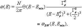 | (13) |
 is a normalization constant chosen so that
  and
and  . For such
  using (4) one finds
  | (14) |
 denotes the integral--exponential function[9, 10].In general one has
  | (15) |
 Making use of the asymptotic expansion of
  [10]
[10] 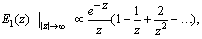 | (16) |
 , one concludes that
 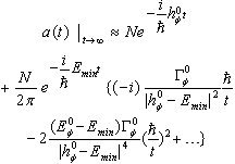 | (17) |
 | (18) |
 (for details see[7]). From (18) it follows that
 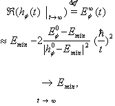 | (19) |
 , and
, and  | (20) |
 | (21) |
 for all densities
  for which the Fourier transform (4) exists. The same can be done for the derivative of
  and then using (6) or (9) a general asymptotic form of
  can be found. It looks as follows
  | (22) |
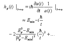
 (compare[8]).Note that from (17) one obtains
 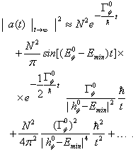 | (23) |
 , where
  denotes the time
  at which contributions to
  from the first exponential component in (23) and from the third component proportional to 1/t2 are comparable. So
  can be be found by considering the following relation Assuming that the right hand side is equal to the left hand side in the above relation one gets a transcendental equation. Exact solutions of such an equation can be expressed by means of the Lambert
  function[11]. An asymptotic solution of the equation obtained from relation (24) is relatively easy to find[12]. The very approximate asymptotic solution,
  , of this equation for
  (in general for
  ) has the form
 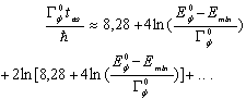 | (25) |
3. Numerical Calculations
- Long time properties of the survival probability
 and instantaneous energy
  are relatively easy to find analytically for times
  even in the general case as it was shown in[8]. It is much more difficult to analyze these properties analytically in the transition time region where
  . It can be done numerically for some models (see[13]).The model considered in Sec. 2 and defined by the density
  , (13), allows one to find numerically the decay curves and the instantaneous energy
  as a function of time
  . The results presented in this Section have been obtained assuming for simplicity that the minimal energy
  appearing in the formula (13) is equal to zero,
  . So, all numerical calculations were performed for the density
  given by the following formula
 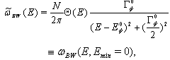 | (26) |
 . Performing calculations particular attention was paid to the form of the probability
  , i. e. of the decay curve, and of the instantaneous energy
  for times
  belonging to the most interesting transition time-region between exponential and non-exponential parts of
  , where the following relation corresponding with (24) takes place,
  | (27) |
 are defined by (15). Results are presented graphically below in Figs (1) - (6).
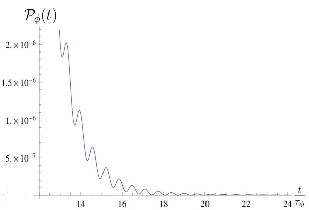 | Figure 1. Survival probability  in the transition time region. The case in the transition time region. The case  |
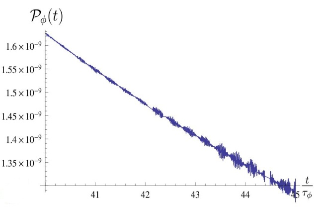 | Figure 2. Survival probability  in the transition time region. The case in the transition time region. The case  for times t longer than those in Fig. 1 for times t longer than those in Fig. 1 |
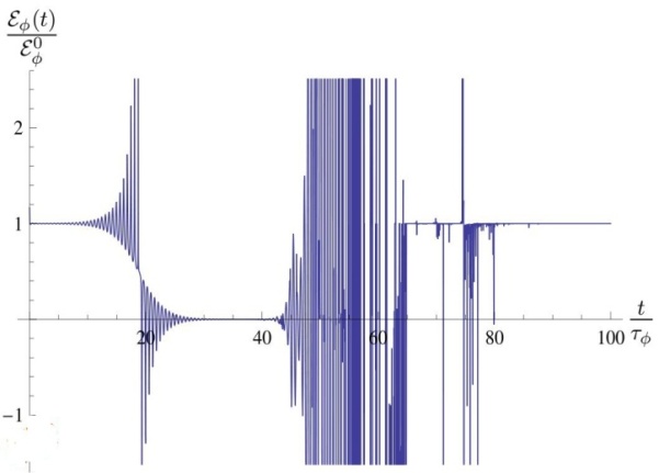 | Figure 3. Instantaneous energy  in the transition time region. The case in the transition time region. The case  |
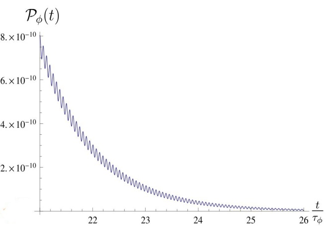 | Figure 4. Survival probability  in the transition time region. The case in the transition time region. The case  |
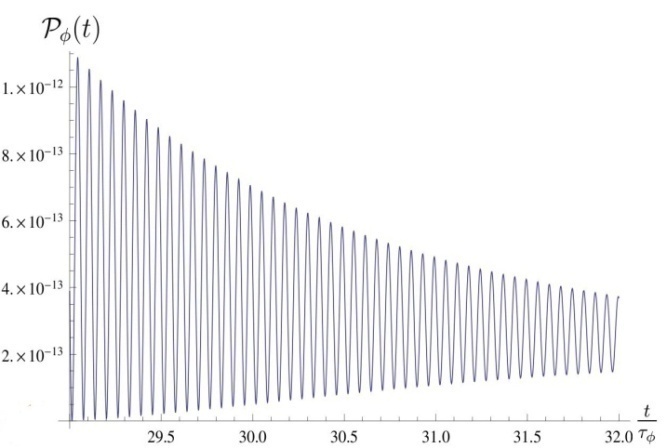 | Figure 5. Survival probability  in the transition time region. The case in the transition time region. The case  for times t longer than those in Fig. 4 for times t longer than those in Fig. 4 |
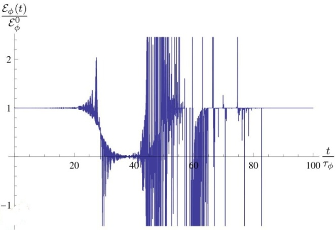 | Figure 6. Instantaneous energy  in the transition time region. The case in the transition time region. The case  |
4. Discussion: Possible Hyphotetical Effects
- Decay curves of type shown in Fig. (1), Fig. (2), Fig. (4), Fig. (5) can be encountered for a very large class of models defined by energy densities
 of the following type (see[2, 14]),
 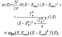 | (28) |
 ,
,  is a form-factor - it is a smooth function going to zero as
  and it has no threshold and no pole. The asymptotical large time behavior of
  is due to the term
  and the choice of
  (see, eg.[2, 8]). The Breit-Wigner part,
  , of the density (28) is responsible for a behavior of
  at exponential decay time region and at transition time region. The density
  defined by the relation (28) fulfills all physical requirements and it leads to the decay curves of a very similar form at transition times region to the decay curves presented above. The characteristic feature of all these decay curves is the presence of sharp and frequent oscillations at the transition times region (see Figs (1), (2), (4), (5)) (see also, eg.[9],[15] -[20]). So derivatives of the amplitude
  may reach extremely large values for some times from the transition time region and the modulus of these derivatives is much larger than the modulus of
  , which is very small for these times. This explains why in this time region the real and imaginary parts of
 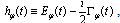 , which can be expressed by the relation (6), ie. by a large derivative of
  divided by a very small
  , reach values much larger than the energy
  of the unstable state measured at times for which the decay curve has the exponential form. For the model considered we found that, eg. for
  and
and  the maximal value of the instantaneous energy equals
  and
and  reaches this value for
 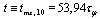 and then the survival probability
  is of order
  .The question is whether and where this effect can manifest itself. It seems that the following two possibilities of observing the above long time properties of unstable states are worth considering: The first one is that one should analyze the properties of unstable states whose
  values are not too big. The second one is finding a possibility to observe a suitably large number of events, i.e. unstable particles, created by the same source and living suitably long.The problem with understanding the properties of broad resonances in the scalar sector (
 meson problem[21]) discussed in[18,22] and recently in[23] where the hypothesis was formulated that this problem could be connected with the properties of the decay amplitude in the transition time region, seems to be possible manifestations of this effect and this problem refers to the first possibility mentioned above. There is the problem with determining the mass of broad resonances. The measured range of possible mass of the
  meson is very wide, 400 - 1200 MeV. So one can not exclude the possibility that the masses of some
  mesons are measured for times of the order of their lifetime and some of them for times where their instantaneous energy
  is much larger. This is exactly the case presented in Fig. (3) and Fig. (6). For broad mesons the ratio
  is relatively small and thus the time
  , when the above discussed effect occurs, appears to be not too long.Astrophysical and cosmological processes in which extremely huge numbers of unstable particles are created seem to be another possibility for the above discussed effect to become manifest. Rapid fluctuations of the instantaneous energy
  (see Figs 3 and 6) of unstable particles
  take place at times
  of order
  . Fluctuations of
  lead to fluctuations of instantaneous masses,
  , of particles
  ,
,  | (29) |
 close to the speed of light c. The energy
  of such moving particles,
  | (30) |
 , should be the same at times
  and at times
  . This follows from the principle of the energy conservation. From relation (30) one can infer that this is possible only when changes of
  at times
  are balanced with suitable changes of
  (i.e. of the velocity
  ). So, in the case of moving unstable particles, rapid fluctuations (changes) of their velocities should be observed at distances
  from their source. It seems to be obvious that astrophysical and cosmological processes are the only sources able to create suitably large number of unstable particles guaranteeing that a part of them survives up to times
  . Therefore an analysis of these processes and observational data connected with them seems to be only chance to find possible effects caused by rapid fluctuations of velocities of unstable particles at late times.It appears that properties of unstable states at times t much later than
  described by the decay law (23) and relations (18), (19) and (22) may be useful when one tries to explain some cosmological processes. The late time behavior of false vacuum decay is an example of such processes[24, 25, 26]. The false vacuum[24,25] is metastable and space areas with false vacuum decay by tunneling to the space area with the true vacuum state. Some space areas with false vacuum can survive up o times
  and then properties of these false vacuum states are described by relations (18), (19) and (22)[26]. At times
  the energy of the false vacuum state should fluctuate very fast according to the results presented in Fig. 3 na 6. This may also affect properties and a behavior of space bubbles with false vacua.Note that all possible effects discussed in this paper are the simple consequence of the fact that the instantaneous energy
  of unstable particles becomes large for suitably long times compared with
  and for some times even extremely large. This property of
  is a purely quantum effect resulting from the assumption that the energy spectrum is bounded from below and it was found by performing a rigorous analysis of the properties of the quantum mechanical survival probability
  .
.