-
Paper Information
- Next Paper
- Paper Submission
-
Journal Information
- About This Journal
- Editorial Board
- Current Issue
- Archive
- Author Guidelines
- Contact Us
Journal of Nuclear and Particle Physics
p-ISSN: 2167-6895 e-ISSN: 2167-6909
2012; 2(3): 42-56
doi:10.5923/j.jnpp.20120203.04
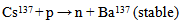
A Calculation Method of Nuclear Cross-Sections of Proton Beams by the Collective Model and the Extended Nuclear-Shell Theory with Applications to Radiotherapy and Technical Problems
 Abstract
 Reference
 Full-Text PDF
 Full-text HTML
1Dept. of Radiation physics, Klinikum Muenchen-Pasing and MPI of Physics, Goettingen, Germany
2Varian Medical Systems, Baden, Switzerland
Correspondence to: W. Ulmer, Dept. of Radiation physics, Klinikum Muenchen-Pasing and MPI of Physics, Goettingen, Germany.
| Email: |  |
Copyright © 2012 Scientific & Academic Publishing. All Rights Reserved.
An analysis of total nuclear cross-sections of various nuclei is presented, which yields detailed knowledge on the different physical processes such as potential/resonance scatter and nuclear reactions. The physical base for potential/resonance scatter and the threshold energy resulting from Coulomb repulsion of nuclei are collective/oscillator models. The part pertaining to the nuclear reactions can only be determined by the microscopic theory (Schrödinger equation and strong interactions). The physical impact is the fluence decrease of proton beams in different media, the stopping power of secondary particles, and a ‘translation’ of the results of the microscopic theory to the collective model.
Keywords: Nuclear Cross-sections of Protons, Collective Model of Nuclei, Extended Nuclear Shell Theory
Cite this paper: W. Ulmer, E. Matsinos, A Calculation Method of Nuclear Cross-Sections of Proton Beams by the Collective Model and the Extended Nuclear-Shell Theory with Applications to Radiotherapy and Technical Problems, Journal of Nuclear and Particle Physics, Vol. 2 No. 3, 2012, pp. 42-56. doi: 10.5923/j.jnpp.20120203.04.
Article Outline
1. Introduction
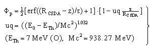
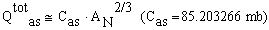
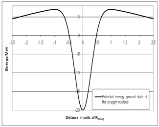
- The accurate knowledge of the total nuclear cross-section Qtot resulting from proton – nuclei interactions is a decisive feature of proton-therapy planning, Monte-Carlo and technical applications. Nuclear cross-sections determine the fluence decrease of primary protons, different ranges and scatter angles of secondary particles (mainly protons and neutrons), passage of protons through materials, and the creation of heavy recoils, which usually undergo β+ decay and emission of γ quanta. Since water represents the usual reference medium for the measurement/calculation of Bragg curves, we consider, at first, the behaviour of Qtot for oxygen, which is the most important case in proton radiotherapy. Figure 1 shows that, for protons, a threshold energy ETh = 7 MeV exists to surmount the Coulomb repulsion of oxygen. At E = 20.12 MeV, Qtot exhibits a resonance maximum and a Gaussian shape in the environment. For E > 50 MeV, Qtot decreases exponentially; at E ≈ 120 MeV, the asymptotic behaviour is reached. The fluence decrease of primary protons Φp[1] can be evaluated by the knowledge of Qtot(E) according to Figure 1:
 | (1) |
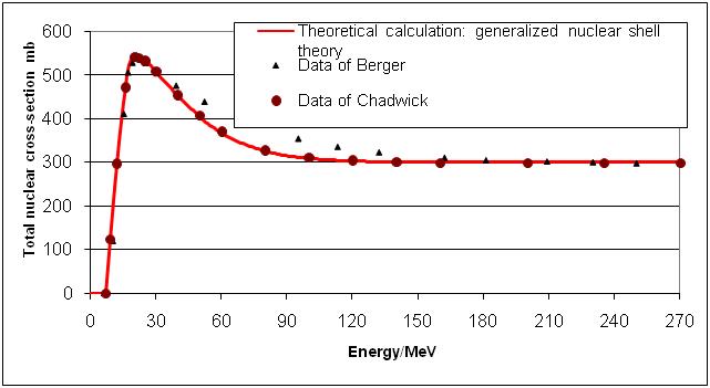 | Figure 1. Total nuclear cross-section Qtot of oxygen[1 - 5] |
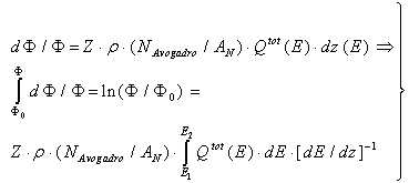 | (2) |
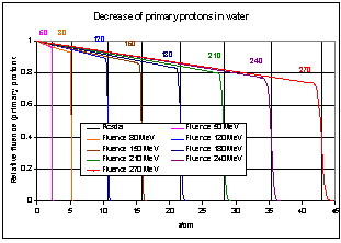 | Figure 2. Decrease of proton fluence in water according to Figure 1 |
2. Theoretical calculation methods of nuclear interactions
2.1. Monte-Carlo Calculations of Energy Transfer, Fluctuations and Multiple Scatter
- The Monte-Carlo code GEANT4 is described in detail in the reference manual [8]. The calculation of the stopping power is based on a numerical manipulation of the Bethe equation with the Bloch corrections (BBE, [9 – 11]). The cut-off amounts to 1 MeV. Since GEANT4 is an open system, all correction terms according to the BBE in accordance with [11] have been implemented. These corrections only imply the removal of singularities, if the total integration procedure is carried out analytically and not by numerical step-by-step calculations of ΔE/Δz; these calculations depend on the actual velocity v and have to be performed for each term of the BBE separately [1]. The scatter of protons is treated by the Molière multiple-scatter theory [12 – 15]. The code also contains a hadronic generator for the simulation of nuclear interaction processes. With respect to proton dose deposition, the basic theory is BBE and a numerical fit of the Vavilov distribution function, which takes account of the Landau tails. In the limit case of fluctuations of small transfer energies from protons to environmental electrons, a Vavilov distribution function assumes a Gaussian shape. In GEANT4, it is also possible to restrict these fluctuations to a Gaussian shape. This fact is of interest with regard to the role of the Landau tails in the initial plateau (entrance region) of Bragg curves. An analysis of Gaussian convolution and its generalizations in physics of protons is given in [5, 16].The accurate knowledge of the total nuclear cross-section Qtot resulting from proton – nuclei interactions is a decisive feature of proton-therapy planning with advanced models and Monte-Carlo calculations. Nuclear cross-sections determine the fluence decrease of primary protons Φp, different ranges and scatter angles of secondary particles (mainly protons and neutrons), collimator scatter, and passage of protons through bones, implants, materials of technical interest, and the creation of heavy recoils, which usually undergo β+ decay and emission of γ quanta. Since water represents the usual reference medium for the measurement/calculation of Bragg curves, we consider, at first, the behaviour of Qtot for Oxygen.
2.2. Nuclear Interactions of Protons, Release of Secondary Protons and Heavy Recoils
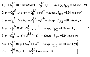
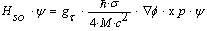
- The most important aspect is the hadronic generator and the energy transport of secondary (and higher-order) particles (protons, neutrons, deuterons, etc.[17 – 21]). However, the default nuclear cross-section implemented in GEANT4 is very poor. Instead of using the default routine, which is based on data of [2], we have implemented the cross-section data of O16 of [4]. Furthermore, we have calculated this nuclear cross-section with the help of the extended nuclear shell theory containing, apart from the strong interaction spin-spin and spin-orbit couplings, the electrostatic interaction and the exchange interactions between the nucleons due to the Pauli principle. Thus, the wave-functions of ground and excited states can be calculated by a perturbed SU3, see [22 – 24]. The calculation of the cross-section due to energy transfer by an external proton is based on well-elaborated principles (determination of the transition probability and density of states). At first, let us return to Figures 1 and 2. The decrease of fluence of primary protons can also be calculated from the results of this figure. Protons with energy lower than the threshold energy ETh cannot surmount the potential wall of O16. Figure 1, which presents the total nuclear cross-section, shows that there is a threshold energy ETh = 7 MeV (more accurate: 6.997 MeV), which a proton should have to perform nuclear interactions with the O16. For proton energies lower than the resonance maximum at Eres = 20.12 MeV, the primary proton is preferably scattered by the nucleus (the secondary proton is now identical to the deflected primary one); the nucleus is excited, to undergo rotations/oscillations and emission of X-rays of very low energy (around 1 keV), leading to the release of Auger electrons. A complete classification of the total nuclear cross-section of the proton – nucleus (O) interaction for therapeutic protons is given by the following two types:1. Potential scatter of protons by the strong interaction potential in the environment of the nucleus (note that Rstrong: ≈ 1.2∙AN1/3 ∙10-13 cm determines a typical distance where the strong-interaction and the Coulomb force ‘balance’ one another; AN = 16). For R > Rstrong, only the Coulomb part is present. Potential scatter accounts for most of the protons undergoing a nuclear interaction. Resonance scattering of the incident protons at the nucleus occurs by inducing transitions between different states of the nucleus (e.g., vibrations leading to intermediate deformations, rotation bands, excited states by changing the spin multiplicity). 2. Nuclear reactions, which produce heavy recoils (see the listing 3 below). These protons are sometimes referred to as reaction protons – or ‘secondary protons’[15 – 21]. For protons in the therapeutic energy domain, the amount of reaction protons is about 1 % - 4.5 %.Within the total nuclear cross-section, the case 1 above plays the dominant role, if the residual proton energy E is lower than 150 MeV. However, for E > 150 MeV case 2 is dominant. In first order, case 1 is described by the Breit-Wigner formula; for a detailed representation of this formula, see[6]. The Breit-Wigner formula results from the exact scatter theory and the restriction of the general S-matrix to ‘S states’, i.e., to l = 0. This restriction is only valid for light nuclei with rotational symmetry. If the number of neutrons is significantly different from the atomic number Z, the related S-matrix has also to account for ‘higher states’, i.e., for l ≠ 0. The total nuclear cross-section obtained by the Breit-Wigner formula has an elastic and inelastic part. The restrictions of the Breit-Wigner formula are insufficient in our problem; an extension to more resonances has been given in [25]. By taking account for the above-mentioned collective vibrations (oscillations of the nucleus by deformations and distortions) and rotations, we have taken into account all these degrees of freedom. Therefore, the total nuclear cross-section shows, around its maximum at Eres, a Gaussian behaviour for E > ETh, before it exponentially decreases to reach the asymptotic behaviour.It has to be added that, in all three cases, about 1 – 7 MeV of the proton energy (depending on the deflection angle) is transferred to whole nucleus to satisfy the energy and the momentum conservation in the center-of-mass system. This implies that for a neutron release, the proton energy has to be 21 – 27 MeV and not simply 20 MeV. Due to the potential barrier, the energy of the colliding proton has, at least, to be 30 MeV in order to release a secondary proton. These two processes have, however, an exception and may also occur at very low energies via exchange of mesons due to the Pauli principle, as pointed out in the discussion of listing (3). The reaction protons (which always result from an inelastic process) are closely related to heavy recoil particles; the most probable heavy recoil elements resulting from the nuclear reactions of therapeutic protons are given by the types (1 – 5); types (6 – 7) result from types (1 – 2).All types of β+-decay emit one γ quantum; its energy is around 0.6 MeV – 1 MeV. The β+-decay of F916 has a half-life of about 20 seconds, and γ quanta are produced by collisions of positrons with environmental electrons. Some of the remaining heavy recoil fragments have half-times up to ten minutes (N15). Since Figure 1 refers to the total nuclear cross-section in relation to the actual (residual) proton energy, we have to add some qualitative aspects to the five different types with regard to the required proton energy: if E < 50 MeV, the type (1) is the most probable case with rapid decreasing tendency between 50 MeV < E < 60 MeV, to vanish for E > 60 MeV. Type (2) also pushes out a neutron, but the incoming proton is not absorbed; the required energy amounts, at least, to 50 MeV. Type (3) is similar, but requires, at least, about 60 MeV, with probability increasing with the energy.
 | (3) |
 | (4) |
 | (5) |
 | (6) |
|
 | (7) |
 | (8) |
 | (9) |
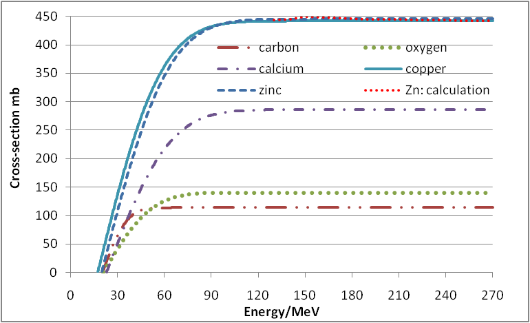
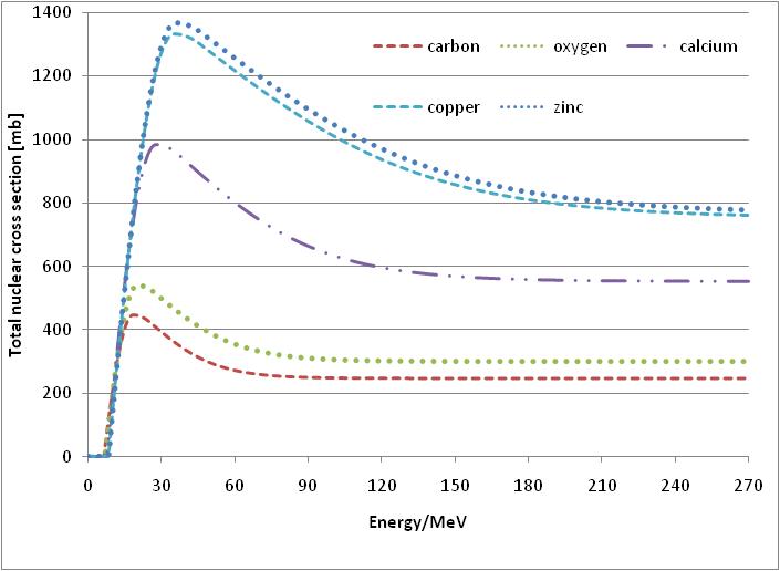 | Figure 3. The total nuclear cross-section for C, O, Ca, Cu, and Zn (taken from [5]) |
|
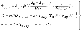
2.3. Secondary Protons Φsp
- In this section, we separate the whole number of secondary protons by their origins, i.e., we differ between reaction protons Φsp,r and non-reaction protons Φsp,n. Due to the complexity the contributions of reaction protons will be determined in a later section.
 | (10) |
 | (11) |
 | (12) |
 | (13) |
 | (14) |
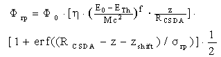
2.4. Recoil Protons/Neutrons Φrp
 | (15) |
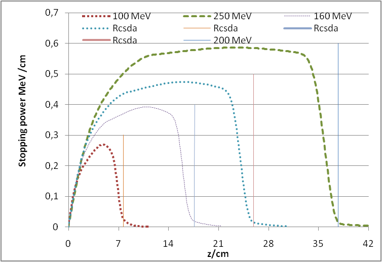
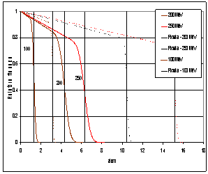 | Figure 4. Decrease of the fluence of 100, 200, and 250 MeV primary protons in copper (solid lines) and in calcium (dashes). The RCSDA ranges are stated by perpendicular lines |
 | (16) |
 | (17) |
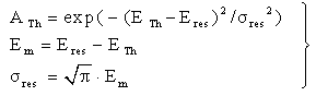
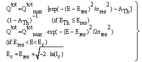
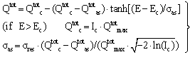
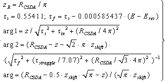
2.5. Fitting Procedure for the Determination of ETh and Qtot
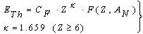
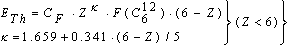
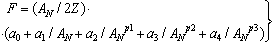
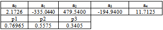
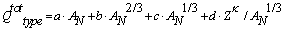
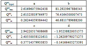
- The calculation of the total nuclear cross section requires some information acquired by fitting the Los-Alamos data, results of extended nuclear shell theory, and empirical rules. Let us at first consider equations (18 – 20) to compute ETh and k. We assume an iso-scalar nucleus, i.e., one in which the numbers of protons and neutrons are equal (AN = 2∙Z). This assumption holds for almost all light nuclei. For nuclei with spherical symmetry, the nuclear radius Rstrong is given by:
 | (18) |
 | (19) |
 | (20) |
 | (21) |
 | (22) |
|
 | (23) |
3. Results of the Generalized Nuclear Shell Theory
3.1 Harmonic Oscillator Models
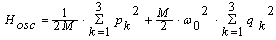
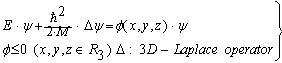
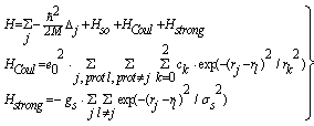
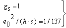
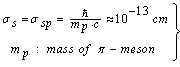
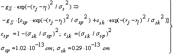
- This section is appropriate only for interested readers. At first, we consider the 3D harmonic oscillator, described by the Hamiltonian Hosc:
 | (24) |
 | (25) |
 | (26) |
 | (27) |
 | (28) |
 | (29) |
 | (30) |
 | (31) |
 | (32) |
 | (33) |
 | (34) |
 | (35) |
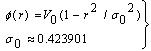
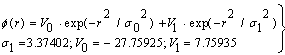
 | Figure 5. Total (effective nuclear potential plus Coulomb repulsion) for O |
 | (36) |
 | (37) |
 | (38) |
 | (39) |
 | (40) |
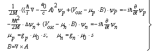
3.2. Nonlinear/Nonlocal Schrödinger Equation, Inharmonic Oscillators with Self-interaction and Hartree-fock Method (Inclusive Configuration Interaction)
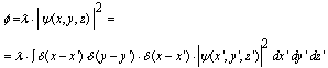
- Let us first consider the usual Schrödinger equation for a bound system:
 | (41) |
 | (42) |
 | (43) |
 | (44) |
 | (45) |
 | (46) |
 is interpreted as a charge density. The Gaussian kernel K also represents the exchange of virtual particles between the nucleons. In view of this fact, we point out that we have incorporated a many-particle system from the beginning. Which information now does this nonlinear/nonlocal Schrödinger equation provide? In order to obtain a connection of the combined equations (44 - 47) with the oscillator model of nuclear shell theory, we analyse the kernel K in detail. In the Feynman-propagator method [32 – 33] the expansion of K in terms of generating functions is an important tool:
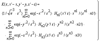 | (47) |
 | (48) |
 (domain with positive curvature), the whole equation is reduced to a harmonic oscillator with self-interaction; the higher-order terms are small perturbations. We summarize the results and refer to previous publications[28 – 31]):
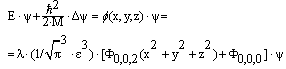 | (49) |
 . This energy level is lowered by the term ~λ ∙Φ0,0,0, depending on the ground-state wave-function. The energy difference between the ground and the first excited state amounts to
  ; this is not true in the case above, since the energy level of the excited states depends on the corresponding eigen-functions (these are still the oscillator eigen-functions!). Next, we will include the terms of the next order, which are of the form ~ λ∙(Φ0,2,2, Φ2,2,0, Φ2,0,2):
 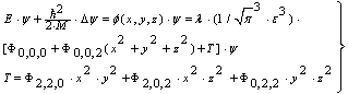 | (50) |
 | (51) |
 acts on the Gaussian kernel K:
  | (52) |
 ) acts on the wave-function. Since the neutron is not a charged particle, the spin-orbit coupling of a neutron can only involve the angular momentum of a proton. In nuclear physics, these nonlinear fields are adequate for the analysis of clusters (deuteron, He, etc.), and has been extended the theory to describe nuclei with odd spin [31]. The complete wave-function Ψc is now given by the product of a function in configuration space Ψ multiplied with the total spin and iso-spin functions. We should like to add that an extended harmonic oscillator model with tensor forces has been regarded in [22]. The application of oscillator models in nuclear physics goes back to [34]. In [32 – 33] it has been verified that the use of Gaussians in the description of meson fields provides many advantages compared to the Yukawa potential (Green’s function according to equation (43)). In a final step, we consider the generalized Hartree-Fock method to solve the many-particle problem. In order to derive all required formulas, it is convenient to use second quantization. The method of second quantization is only suitable to derive the calculation procedure: extension of the Pauli principle to iso-spin besides spin, inclusion of spin-orbit coupling, and exchange interactions. This is the consequence of dealing with identical particles, in which case every state can only occupy one quantum number. In order to get numerical results (i.e., the minimum of the total energy of an ensemble of nucleons, the extraction of the excited states, the scatter amplitudes, etc.), we have to use representations of the wave-function by at least one determinant in the configuration space. In the ‘language’ of second quantization of fermions, we would have to regard expressions like:
 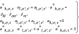 | (54) |
 | (55) |
 | (56) |
 | (57) |
 | (58) |
 | (59) |
 | (60) |
 | (61) |
 | (62) |
 | (63) |
 | (65) |
 | (66) |
 | (67) |
 | (68) |
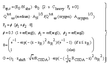
4. Applications to Reaction Protons of the Inelastic Cross-section Ssp,r
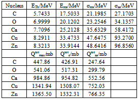
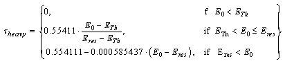
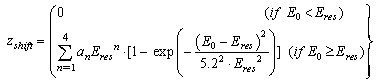
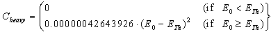
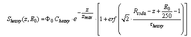
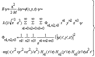
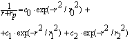
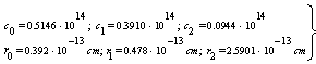
- We have already pointed out that the main purpose for calculations with the extended nuclear shell theory incorporate nuclear reaction contributions of protons, neutrons and further small nuclei to the total nuclear cross sections of nuclei discussed in this presentation. We should also mention that the default calculation procedure of nuclear reactions in GEANT4 is an evaporation/cascade model, which has been developed on the basis of statistical thermodynamics. Figures 2 - 4 do not yet provide final information about the contributions Ssp,n and Ssp,r. The first case of non-reaction protons has already been treated. According to Figure 6 the contribution of reaction protons is particular important for E > 150 MeV with increasing energy. We now present the calculation formulas for this case. Thus Ssp,r is proportional to Φ0∙2∙υ∙Cheavy and a function Fr, depending on some further parameters. It should be mentioned that the parameters of equations (21 - 23) require modifications to be valid for various types of nuclei. However, from Figure 5 the corresponding parameters of some further nuclei can be verified, e.g., ETh, Eres, and some necessary information on the total cross-section. We use the following definitions and abbreviations:
 | (69) |
 | (70) |
 | Figure 6. Stopping power of reaction protons (medium: water) in dependence of the initial energy E0 |
 | Figure 7. Nuclear reaction part of the cross-sections of the nuclei C, O, Ca, Cu and Zn |
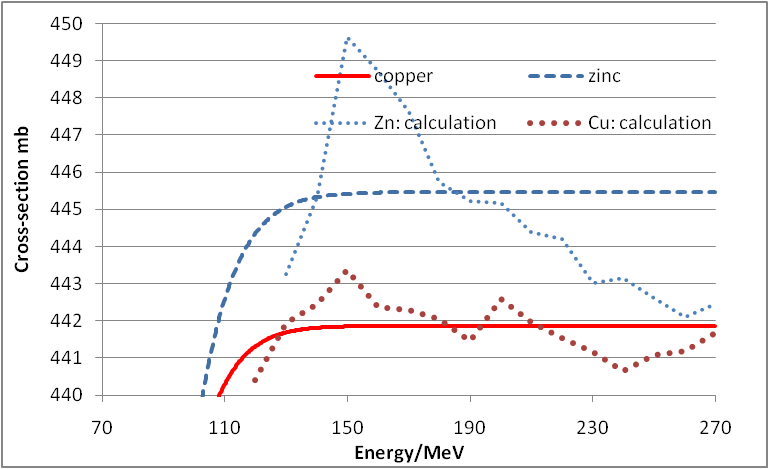 | Figure 8. Calculated cross-sections for Cu and Zn and smooth curves |
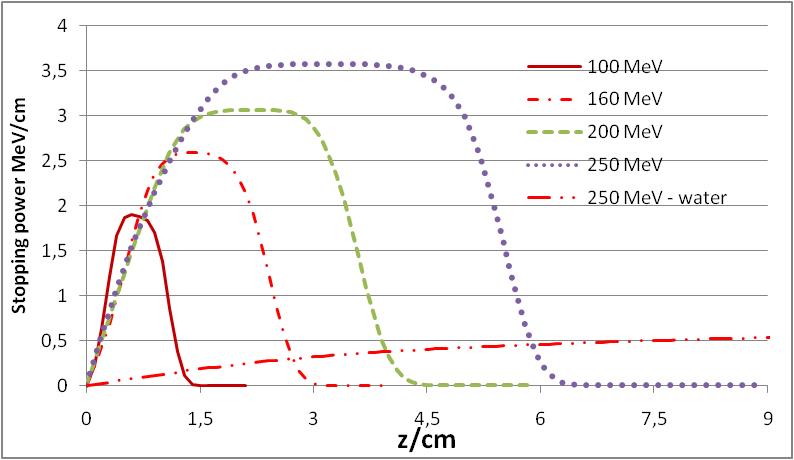 | Figure 9. Stopping power (proton - copper and comparison with water) of secondary/tertiary protons for the initial proton energies 100 MeV, 160 MeV, 200 MeV and 250 MeV |
 | (71a) |
 | (71b) |
 | (71c) |
 | (71d) |
 | (71e) |
 | (71f) |
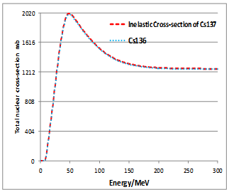 | Figure 10. Nuclear cross-section of the both nuclei Cs137 (dashes) and Cs136 (dots) |
5. Conclusions
- The presented results show that a suitable combination of the collective model with extended nuclear shell theory can be adequate to solve problems, which are rather outstanding in many practical problems. Besides the radiotherapy with protons it should be mentioned that the cross-sections of those nuclei/isotopes are important to reduce the half-times of the corresponding isotopes significantly. The storage of long-existing isotopes should be avoided. However, a discussion of technical details of these processes goes beyond the scope of this study.