-
Paper Information
- Paper Submission
-
Journal Information
- About This Journal
- Editorial Board
- Current Issue
- Archive
- Author Guidelines
- Contact Us
Journal of Mechanical Engineering and Automation
p-ISSN: 2163-2405 e-ISSN: 2163-2413
2023; 12(1): 6-19
doi:10.5923/j.jmea.20231201.02
Received: Mar. 2, 2023; Accepted: Mar. 13, 2023; Published: Mar. 16, 2023

The Numerical Analysis of Single Degree of Freedom Vibration System with Non-Linearity
 Abstract
 Reference
 Full-Text PDF
 Full-text HTML
J. Alrajhi1, K. Alhaifi1, M. Alardhi1, N. Alhaifi1, J. Alazmi1, A. Khalfan1, K. Alkhulaifi2
1Automotive and Marine Dept., College of Technological Studies, PAAET, Kuwait
2Mechanical Power and Refrigeration Dept., College of Technological Studies, PAAET, Kuwait
Correspondence to: J. Alrajhi, Automotive and Marine Dept., College of Technological Studies, PAAET, Kuwait.
| Email: |  |
Copyright © 2023 The Author(s). Published by Scientific & Academic Publishing.
This work is licensed under the Creative Commons Attribution International License (CC BY).
http://creativecommons.org/licenses/by/4.0/

A numerical analysis of a Single Degree of Freedom Vibration (SDOF) vibration system with non-linearity is investigated. Mag-spring as a nonlinear spring with hardening behaviour is added in parallel to a vibrating system. The nonlinear effect is expected to curve the vibration amplitude and shift away the system’s natural frequency only where it is necessary. Due to hardening behaviour of the nonlinear Mag-spring especially at higher amplitudes, nonlinearity kicks in and the stiffness of the system is increased; then the natural frequency of the system is shifted to a higher value away from the excitation frequency. It has been shown that how a light damping could lead a forced vibration system to a steady state. Moreover, it explains how a nonlinear spring can be fitted in parallel to the main system with one degree without changing its degree of freedom. The techniques utilised to formulate the equation of non-linear spring have been explained as well. Based on the characteristics of the nonlinear spring, a system with appropriate parameters has been formulated. Further, a second order nonlinear differential equation is solved by a written program in MATLAB software. It shows how the initial conditions and the differential equation in a state space form will be used by ode45 function in MATLAB to solve the system.
Keywords: Single degree of freedom, Vibration, Mag-spring, MATLAB
Cite this paper: J. Alrajhi, K. Alhaifi, M. Alardhi, N. Alhaifi, J. Alazmi, A. Khalfan, K. Alkhulaifi, The Numerical Analysis of Single Degree of Freedom Vibration System with Non-Linearity, Journal of Mechanical Engineering and Automation, Vol. 12 No. 1, 2023, pp. 6-19. doi: 10.5923/j.jmea.20231201.02.
1. Introduction
- High line speeds can result in thermal distortion in the shift clutch of the vehicle transmission system, which will generate vibration and have a significant impact on the performance of the friction element and other related components. The design of the clutch of a vehicle power-shift steering transmission system depends heavily on the thermal deformation of the friction pairs and its vibration. As a result, it has important theoretical and engineering ramifications to thoroughly examine the vibration appearances of the friction pairs at high line speed and to advance the development of a practical vibration control system. A microscopic normal element contact model of thermal distortion is recognised by appertaining the theory and technology of surface structure characteristics and contact mechanics of friction pairs from the belvedere of micro mechanics. The link between micro and macro is then established, making full use of statistical statistics and standardisation techniques. Thus, a mathematical model of macro contact between two pairs of frictional pairs is obtained. The viscoelastic contact property including stress and strain is constructed at the same time as the Kelvin-Voigt model is presented and the viscoelastic contact differential operator is developed into a mathematical model, allowing for the creation of a viscoelastic contact mathematical model of the friction pairs. Finally, mechanical analysis yields the mathematical model of nonlinear vibration, and its vibrational features are simulated. The accuracy of the simulation model is confirmed by testing the nonlinear vibration characteristics with varying rotational speed and lubricant. By adopting a magnetorheological (MR) fluid damper, key, and subharmonic concurrent resonance for the Duffing-type nonlinear system under base innervation and external innervation is passively controlled. The fractional-order derivative Bingham model of MR fluid damper is assessed in this study. The incremental averaging method is used to arrive at the system's approximated logical solution.Based on gaining the principal resonance of the system under base innervation by the averaging method, the subharmonic resonance solution of the system is obtained by taking the subharmonic resonance of the system under base innervation and external innervation as an increase, to obtain the estimated analytical solution of the concurrent resonance of primary and subharmonic resonance. And the amplitude–frequency equation and phase–frequency equation of the steady-state solutions for the primary and subharmonic resonance of the system are derived respectively. According to the approximate analytical solutions, the steadiness conditions of the steady-state solution of the primary resonance and subharmonic instantaneous resonance are obtained by Lyapunov method. Hence, it becomes necessary to study latest improvements in oscillating isolators applied in various applications. A review has been carried out by scholars Alkhatib & Golnaraghi [1] to achieve structural vibration control. Several scholars—namely Symans & Constantinou [2], Chu et al. [3] and Casciati et al. [4] have performed research efforts concerning the development and utilisation in semi-active structural control system for vibration reduction applications. Passive control systems have undergone various changes in order to enable adjustments to be made in regard to the mechanical aspects; these are considered to be the benchmarks from which semi-active systems originate. Semi-active vibration control systems offer most performance characteristics of active systems, and they don’t require large power sources. Moreover, they are not a threat to destabilize the system, and that because they don’t inject energy into the controlled system [2,5,6]. A comprehensive coverage of the theory of linear vibration isolation was provided by Crede [7], Snowdon [8] and Rivin [9]. Tuned Vibration Absorbers (TVA) was pioneered by Watte [10] and Frahm [11]. As stated by researchers, by increasing the damping ratio, working range of the main system becomes wider (positive point), however the magnification ratio increases negative point as well. Since, the first mathematical model was proposed by Ormondroyd and Den Hartog [12], huge investigations have been carried out in the past years to introduce new models for passive TVAs that could solve the off-tuning problems. Among the latest, Liu and Coppola [13], offered an optimal design for a damped linear vibration absorber including a new combination of the mass and damping as well. The fundamental idea behind vertical and horizontal motions were estimated by Winterflood et al. [14]. Dynamic anti-resonant vibration isolators are another class of linear isolator introduced in the literature by Goodwin [15], Halwes [16] and Flannelly [17]. Goodwin and Halwes [15,16] emphasise that anti-resonant isolators are based on hydraulic leverage, although the isolator of Flannelly [17] is based on a levered mass. The levered mass lowers the resonant frequency of the isolator, which accordingly enhances its overall ability to operate at a lower frequency range. This type of anti-resonant is used in an isolation helicopter rotor and floor machines [18-21]. The rubber engine mounts were replaced with hydraulic engine mounts by Corcoran & Ticks [22] and Flower [23] and comprise what is referred to as inertia track property; notably, there are several similar components between the frameworks of Goodwin and Halwes [15,16]. Yilmaz & Kikuchi [24,25] investigated the theory of anti-resonant vibration isolators, comprising various degrees of freedom regarding passive isolators comprising at least two anti-resonance frequencies.The effect of a non-linear isolator on the communicable, relays in particular regard on its inflexibility if it is flexible or firm [26]. when considering the suspensions’ response regarding high-speed vehicle and fragile instruments’ mounts—non-linearity becomes essential to be considered [27]. Hundal & Parnes [28] studied a vibration system when under base oscillation. Moreover, Metwalli [29] introduced a design centred on enhancing and improving the suspension systems non-linear in nature, that accordingly established to perform better than their opposite linear systems. Nayfeh et al. [30] and Yu et al. [31] investigated mechanical passive vibration isolators, incorporating distinct damping, mass, and stiffness aspects, highlighting that the more confined non-linear styles may be incorporated within the system through the proper design of the system’s stiffness non-linearities. Popov & Sankar [32] proposed a non-linear orifice type damping comprising a changing damping coefficient, which is regarded as an interior geometry function, flow fluctuation frequency, and Reynolds number.Vibration control methods have been classified into three areas, namely passive, active or hybrid (active/passive) methods. Overall, the techniques accepted for vibration control in the context of industrial equipment comprise damping, force reduction, mass addition, isolation, and tuning the system’s natural frequency. Many scenarios and case studies have been introduced, with emphasis placed on the tuning of the natural frequency as a method to avoid resonance or postpone from the working frequency of the system. Latest developments in metallic and viscoelastic non-linear vibration isolators have been provided with covering classical and non-classical systems. The major characteristics of non-linear isolators were explained. These characteristics contain the shifting of the resonance frequency, jump phenomena, chaotic motion, and internal resonance. The transmissibility curves of non-linear isolators subjected to non-harmonic force require explanation regarding the mean squares of response, as well as excitation amplitudes. Viscoelastic non-linear isolators offer various mechanical features owing to their stiffness and damping parameters dependence on frequency and temperature. As has been well documented, the vibration amplitude of the non-linear viscoelastic isolator is known to increase in line with the reduction of the response amplitude, and the transmissibility is improved over that of the linear isolator for vibration frequency, which exceeds a specific value governed by the temperature and excitation amplitude. The literature survey has shown that non-linearity has been utilised widely in terms of controlling vibration by many people. Therefore, this research will investigate non-linearity in vibration control. Several examples have been brought from the literature. The major element noticed in using non-linearity in the past was the fact that, these non-linearities were mechanically designed, structurally fixed, and difficult to modify. Therefore, designing a non-linear spring to give vibration characteristics was a very difficult task.However, the developments in regard of the magnetic spring technology have supported the idea that non-linearity can now be designed to specifications using magnetic technology. Therefore, the idea of studying the use of magnetic technology in terms of developing a non-linear spring, and using it in vibration control, is a thought that has come to mind.This research proposes a new idea that has the potential to lead to overcoming the previously mentioned shortages. The improvements in terms of magnetic technology have encouraged this research with the new invented Mag-spring (magnetic spring explained in the next chapter). The Mag-spring was invented for a purpose other than vibration cancelation. However, the non-linearity that Mag-spring shows brought the idea of investigating a new way that could guide to a novel point of view in enhancing the vibration cancellation in vibrating structures.
2. Research Methodology
- Hardening non-linearity is used for design of vibration based on single degree of freedom system. the effect of non-linearity on vibration characteristic was studied here. Mag-spring was chosen to represent the non-linearity in the system. Mag-spring is a totally passive device that consists of two permanent magnets (introducing the attractive force) as a slider and a stator sliding against each other while separated and guided by a plain Teflon as a bearing as shown in Figure 1.
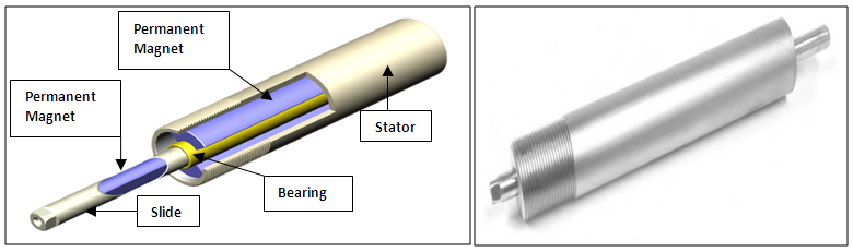 | Figure 1. Magnetic spring to provide non-linearity (www.linmot.com) |
3. Results and Discussion
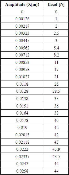
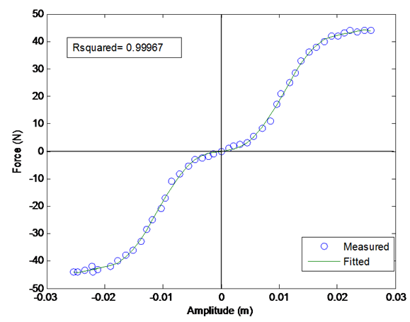
- 1. Load Deflection Experiment of the SpringThe rational of selecting a nonlinear spring is explained above and as it will be demonstrated, the spring will provide the required behaviours both for hardening and softening. To start developing the simulation model, the stiffness curve of the spring will be used in mathematical models from the outset. In the experiment, the applied loads are varied to observe the extension of the spring. For every applied load, the extension is recorded and tabulated as shown in the Table 1. Based on recorded data, a non-linear regression equation has been established using curve-fitting technique.
|
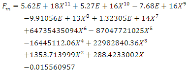 | (1) |
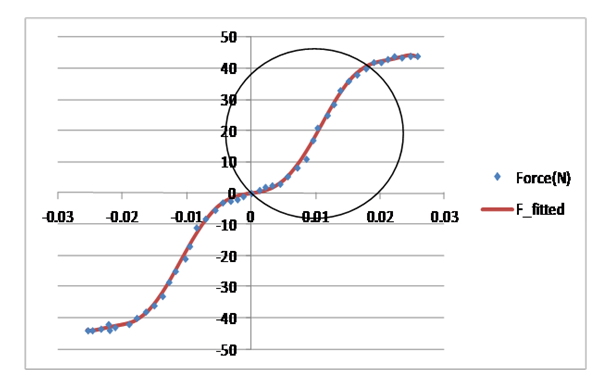 | Figure 2. Fitting of Curve |
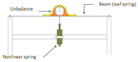 | Figure 3. Proposed vibration system |
 | (2) |
 | (3) |
 | (4) |
 and
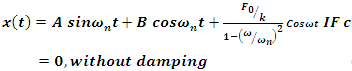
and 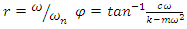 The unknown coefficient in the complementary part of equations 3 and 4, A and B, are determined by forcing the initial conditions. Applying initial condition for the undamped system:
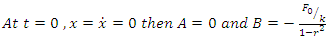 Finally,
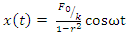
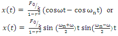 | (5) |
 or
or  the beating phenomena (Figure 4, left) with the beating period of
  will happen. However, when
  or
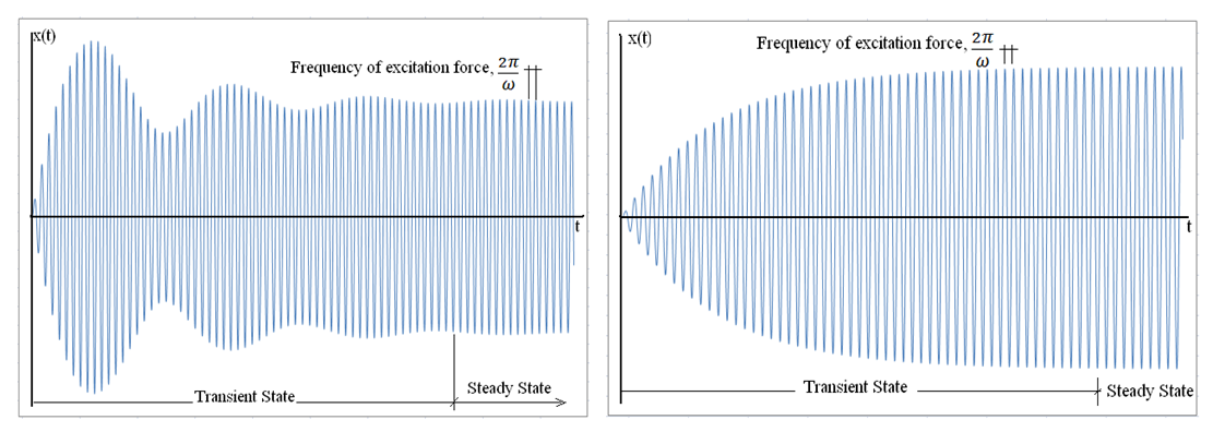
or  the beating frequency and amplitude go to infinity (Figure 4, right). The vibration amplitude keeps increasing and this phenomenon is called resonance. This is the reason when designing a system, the system’s natural frequency should be estimated with keeping in mind that excitation frequency should not go near the natural frequency of the system. Therefore, shifting the natural frequency away from the excitation frequency is done by adding nonlinear stiffness to the main system.
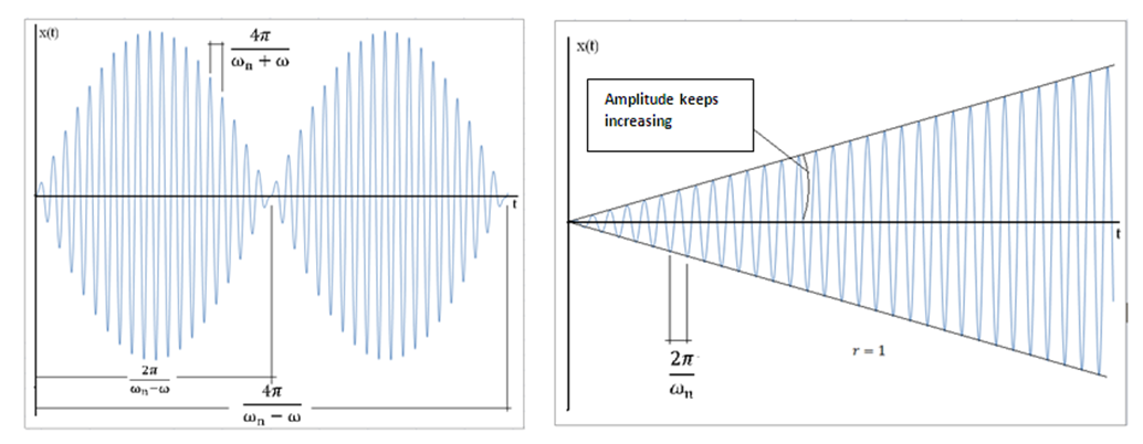 | Figure 4. Response of a linear single degree of freedom system with forced vibration. Left, frequency of excitation is different from natural frequency of the system  Right, frequency of excitation and natural frequency of the system are equal Right, frequency of excitation and natural frequency of the system are equal  |
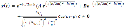
 represents the exponential decaying function of time. However, the behaviour of the term
 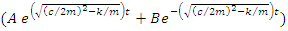 depends on the numerical value of the
  (under the radical); if it is positive, negative or zero. When damping term
  is larger than
  , the radical become positive, then exponents in the Eqn. 4 become real and no oscillation is possible. This situation is called overdamped response. On the other hand, when damping term
  is smaller than
  the radical become negative, then exponents in the Eqn. 4 become imaginary number and oscillations are possible. This situation is called underdamped response. If damping term
  is equal to the
  radical become zero. This situation is called critical damping,
  response:
 | (6) |
 According to Figure 5, for the cases where the damping ratio is less than ζ < 0.1 although the system is underdamped, the damping does not have much effect on the response of the system. For instance, if the system with mass,
  Stiffness
  = 10000N.m, natural frequency is
 ; if we define damping ratio ζ = 0.01 and
  ; then damping coefficient,
  in the Eqn.4.1 becomes
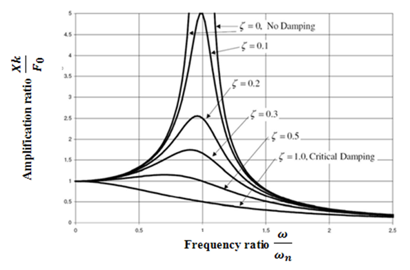 | Figure 5. Diagram of Amplitude ratio verses Frequency ratio for a forced vibration system – the response of system at different damping ratio (Tustin 2006) |
 | (7) |
 | Figure 6. Light damping on a system with forced vibration, 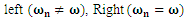 |
 Free body diagram of the system has been shown in Figure 7(b). The force conducted by nonlinear spring is shown by
  The force created by the linear spring is
  Based on Figure 44 (b), the equation of the system can be derived as follows:
 | (8) |
 To solve the equation a numerical method has been used. The use of MATLAB to compute the solution of the equation and the results of the simulation will be shown in the following section.
 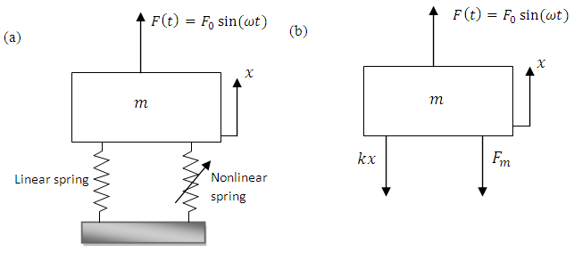 | Figure 7. (a) nonlinear spring was added in parallel to a system with one degree of freedom. (b) Free body diagram of the system with nonlinear stiffness |
 | Figure 8. Curve fitting |
 in non-linear vibration system model. The nonlinear differential equation does not have an analytical solution, hence, to find the response of this equation in time and frequency domain a program in MATLAB software was prepared. MATLAB softwareThe equation 8 has been developed to model a SDOF vibration system. This is a nonlinear second order differential equation and there is no straight forward analytical solution for this equation. Therefore, in this work, the solution for this equation will be computed in a numerical analysis with the aid ODE45 function in MATLAB Software.ODE45 FunctionTo solve the non-linear vibration equation obtained and displayed in equation 8, a separate function of
  is built and this function will be called an ordinary differential equation solver, ODE45 using MATLAB. This routine utilizes a variable step fourth order Runge-Kutta Method with 5th order corrector in solving differential equations numerically as follows:[t,x]= ode45 (@my_function,[t0,tf],[x0,xdot0]),where “my_function” is a Matlab function
  which has been used to introduce the nonlinear differential equation while, t0 introduces the initial time, the final time is tf and x0 is the initial displacement and the initial velocity is xdot0. The results of the differential equation are stored in an array called x, which contains in its first column the values of amplitudes and in the second column the corresponding values of velocities, x[x, xdot].Initial conditionThe system is assumed to start from the rest position, where displacement
  and initial velocity,
  The initial condition should not be out of the operating range.%initial conditions x0=0; %displacementxdot_0=0; %velocityState space variablesTo use the ode45 function, it is essential to write the differential equation in state space form.xdot1=x(2);xdot2=-k1/m1*x(1)-1/m1*(a11*x(1)^11+a10*(x(1))^10+a9*(x(1))^9+a8*(x(1))^8+a7*(x(1))^7+... a6*(x(1))^6+a5*(x(1))^5+a4*(x(1))^4+a3*(x(1))^3+a2*(x(1))^2+a1*(x(1))+a0)+1/m1*F0*sin(w*t)-ldamp*x(2)/m1;xdot=[xdot1;xdot2];In the above functions the x(1) and x(2) are the x array components, which shown displacement and velocity, respectively. Xdot1 and xdot2 are the first and the second differentiation of the displacement (velocity and acceleration).Frequency domainAmong the key code in programming the model of the vibration system is to determine the maximum amplitude for every frequency set. Since the time constants are dependent to the iterations done in ODE45 function, the array of the highest amplitude varies from one frequency to another. Therefore, a dynamic loop is developed to search the highest value in an array and stores it in an exclusive maximum amplitudes array, x_n(i), and this array can be used to plot a graph for maximum amplitude against frequency later. The time of when this maximum amplitude happens is also recorded for verification. The important issue is to make sure the maximum amplitudes are selected from the steady state parts of the time domain. To find the steady state response it is possible to check the convergence of the results to meet a minimum difference between two consecutives maximum. Also, it is possible to let the program runs for a longer time; then to pick the maximum after a specific time which certainly the results have been converged. In this program, it has been checked that the steady state will happening after 5s in real time domain which is equivalent of 2500 steps in time (in ode45 function dt=0.002s). The code to search the highest amplitude in an array is written below.
 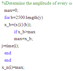 Parametric studyTo show how nonlinearity could improve the behaviour of a system with one degree of freedom at a forced vibration system (especially when the excitation frequency is near the natural frequency of the main system), a spring with nonlinear behaviour has been introduced. This nonlinear spring has a hardening/softening behaviour. At low amplitude of vibration this spring shows hardening behaviour, which means at the beginning it has very low stiffness and gradually it will increase by increasing the amplitude of vibration. As a result, the nonlinear spring at low amplitude of vibration does not affect the main system very much which is desirable. On the other hand, when the amplitude of vibration is increased (resonance) the nonlinear spring shows higher stiffness and shifts the natural frequency of the system out of the excitation frequency range.Defining the main system parametersTo choose a main system (stiffness and mass) which is suitable for our nonlinear spring, a series of runs have been performed. At the first stage, a system with natural frequency
  was chosen and the nonlinear spring was added to the system (in parallel); then a set of runs were defined. The stiffness and mass of the main system were changing in a way to keep constant natural frequency of the main system. Figure 9 shows that the nonlinear stiffness is more effective for the system with lower stiffness and mass at constant natural frequency
 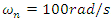 . This could be predicted as the nonlinear spring will add to the stiffness of the main system and the system becomes stiffer (without increasing the mass of the system); this issue is not recommended for the frequencies lower than natural frequency of the main system as to make the system stiffer were it is not really necessary, however it will help to shift the resonance to higher frequencies which is desirable.
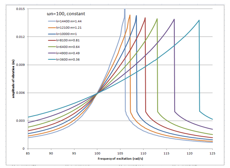 | Figure 9. Amplitude of vibration verses frequency of excitation (frequency domain) for constant natural frequency of the main system with different stiffness and mass |
 with different stiffness. As a result, the natural frequency of the main system was not constant. Series of runs for this case have been performed; the results have been shown in Figure 10.
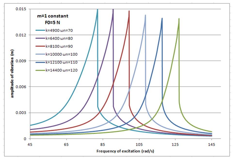 | Figure 10. Amplitude of vibration verses the frequency of excitation. Mass of the main system is constant however the stiffness of the main system is different for each set of data |
 | Figure 11. Amplitude of vibration verses the frequency of excitation. Stiffness of the main system is constant however the mass of the main system is different for each set of data |
 =10000N/m and
  will be a proper main system.Defining the excitation force parametersAnother important parameter in forced vibration analysis is the amplitude of excitation
  . The magnitude of
  should be limited; otherwise, the excitation force is beyond the system capacity. Also, the introduced nonlinear spring has a limited working range (±0.03m, see Figure 45). To maintain in the specific limits a series of runs has been performed for a system with
 and ζ=0.01 at various
  . Figure 12 shows that if the
  goes beyond 15 N the amplitude of vibration for some frequency near the natural frequency goes to infinity. As a result, the
  =5N has been chosen to ensure the system does not fail in the specific frequency.
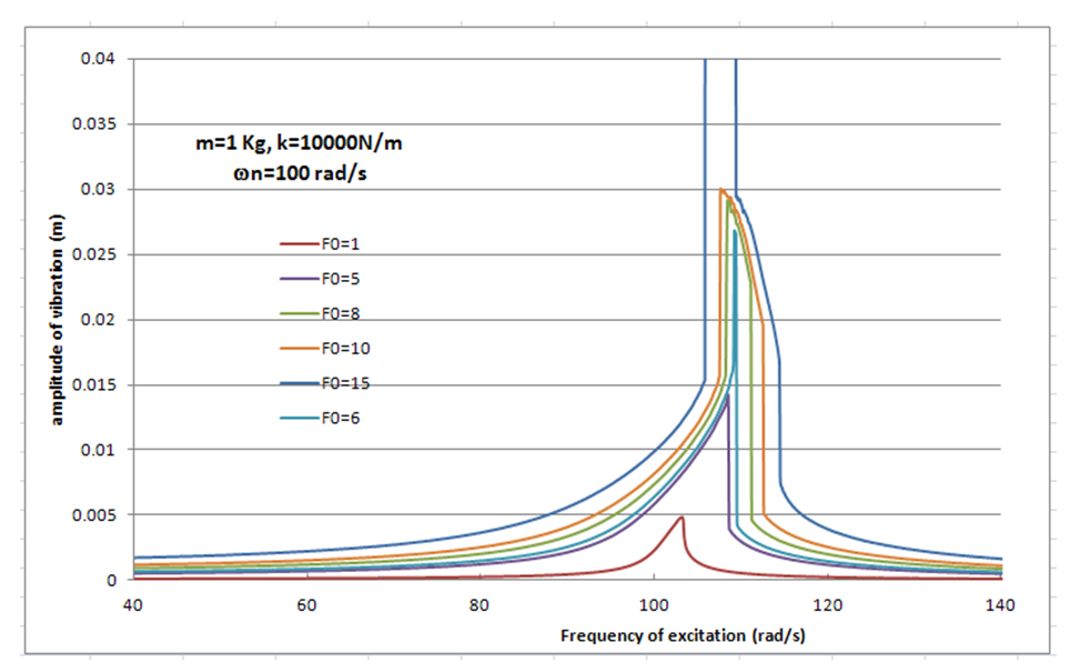 | Figure 12. Amplitude verses Frequency of excitation for different excitation amplitude for different magnitude of excitation force, damping ration maintain constant ζ=0.01 |
 and stiffness
  has been chosen; The simulation results for amplitude of excitation force
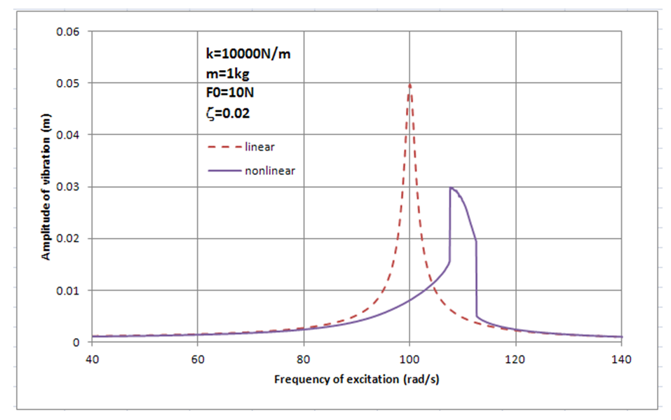
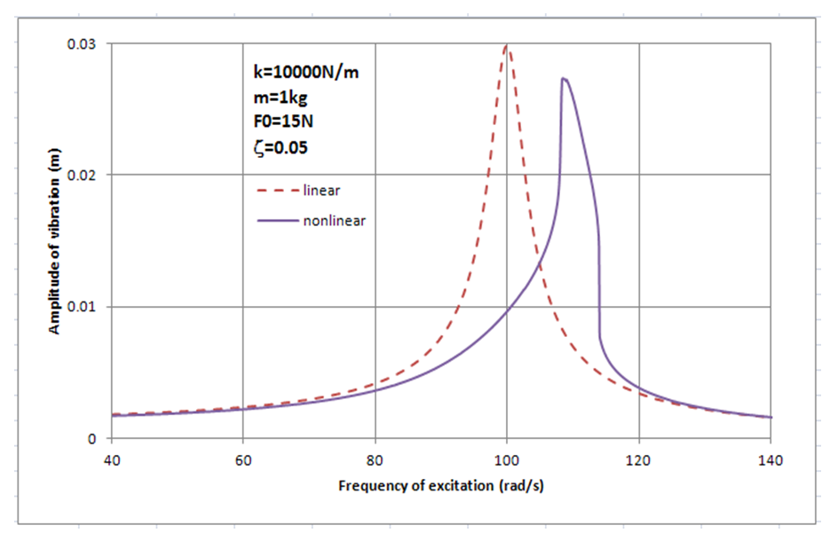
  =5N, 10N, 15N, 20N, and damping ratio ζ=0.01, 0.02, 0.05, 0.1 has been done, respectively and the behaviour of the main system has been studied in two different conditions. In the first scenario the main system was under an excitation force with constant amplitude,
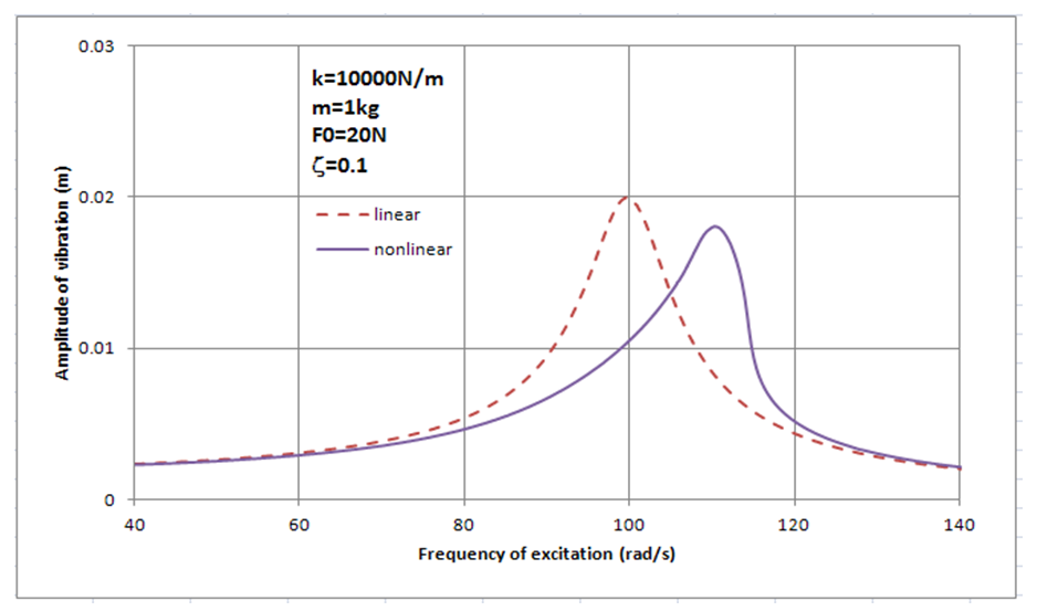
  , constant light damping, ζ, and variable frequency from 40rad/s to 140 rad/s. In the second scenario, a nonlinear spring has been added in parallel to the main system as an absorber. Then, the results of a system with non-linear stiffness compared with the results of the main system (without the absorber). Figure 13 to Figure 14 show the results of simulation for the main system with and without the nonlinear spring. According to the graphs the nonlinear spring will cause to shift the frequency by about 10%. Also adding a hardening nonlinear spring will not make the system stiffer in the frequencies lower than the natural frequency of the main system. Moreover, the nonlinear spring decreases significantly the amplitude of vibration at the natural frequency of the main system in the systems with very low damping and low excitation force. In addition, in the response of the system with nonlinear spring, there is an excitation frequency that provides two different amplitudes of vibration in the same frequency (one of them is the maximum amplitude) which is an expected response of a hardening spring.
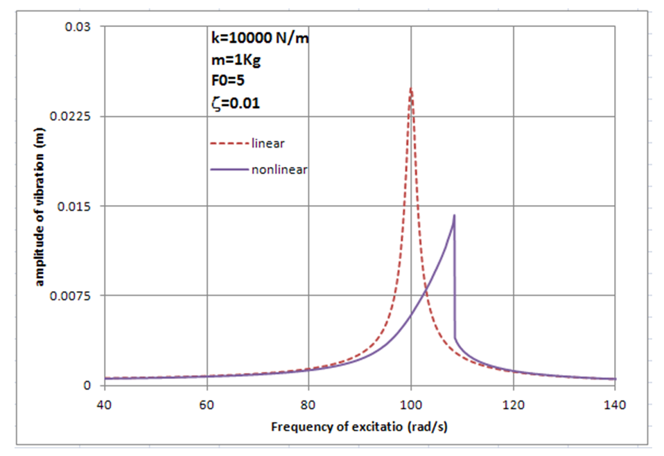 | Figure 13. Amplitude verses frequency of excitation for the main system with and without nonlinear stiffness.  |
 | Figure 14. Amplitude verses frequency of excitation for the main system with and without nonlinear stiffness.  |
 | Figure 15. Amplitude verses frequency of excitation for the main system with and without nonlinear stiffness.  |
 | Figure 16. Amplitude verses frequency of excitation for the main system with and without nonlinear stiffness.  |
 which is rotating with angular velocity of
  In this case,
  is not anymore constant and replaced with the
  In this case the response of the system with and without the nonlinear spring has been compared as well. In the unbalance rotating machine as the amplitude of the excitation force is changing by frequency of excitation,
  the unbalance parameters should be designed in a way to maintain the system in a working range of nonlinear spring. As in the natural frequency of the system, the excitation has maximum affect; suppose
  is 12N at natural frequency of the system
 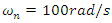 then
then  or
or  and
and  Figure 17, shows the response of the main system
  to the excitation force due to the unbalance mass
  with eccentricity of
  =0.04m for different light damping. As it can be seen from the graphs that the damping ratio lower than 0.02 is not suitable for this simulation as the results going to infinity before reaching to the steady state. In addition, the amplitude of vibration for the system with nonlinearity is slightly higher than the linear systems; due to the nature of the unbalance force which will increase by excitation frequency. In the next chapter, the above simulation results will be tested for a specific case.
  | Figure 17. Amplitude of vibration verses the Frequency of excitation, for the main system  |
 = 12N at the spring natural frequency
  =100rad/s; an unbalance mass,
  and eccentricity of
  will be needed as
 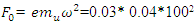 =12 N.
 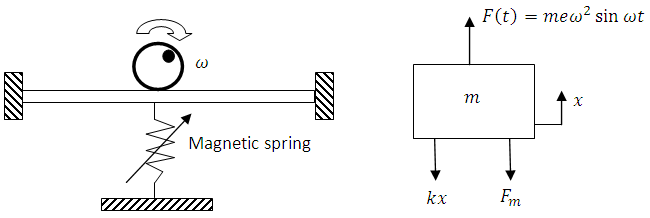 | Figure 18. Proposed system schematic and free body diagram |
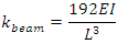 The equivalent mass of the system = total mass +beam equivalent mass.
4. Conclusions
- In this research paper a single degree of freedom systems with linear undamped vibration and non-linear undamped vibration were modelled and numerically simulated. The programming environment chosen for the simulation is MATLAB, due to its capabilities to simulate the models numerically and yields the results graphically. The reliability of the model is initially tested and verified by determining the frequency at where the resonance occurs in linear vibration system. The correlations gained between the simulation and theoretical calculation allows the code to be used further to simulate the linear and non-linear undamped vibration models. A parametric study has been performed to find out how the nonlinear spring is responding to the forced vibration amplitude in the main system. There are some distinct differences observed in analysing the parametric study. Firstly, it is observed that the resonance of the system is shifted away from about ten percent when a non-linear component is added to vibration system. Secondly, the behaviour of the system response curve has changed due to the nonlinearity, that curved the system’s high amplitude and forcing it down. The resonances are detected at a higher frequency in non-linear model.To validate the results of the simulation an experimental setup has been built for a forced vibration system due to unbalance mass. In the next chapter it has been shown how the experimental set up has been designed. The information obtained in the numerical analysis will be used in designing the experimental setup especially in determining the domain and resolution of sensing and data acquisition equipment.