1. Introduction

Space system guidance and control algorithms need a source of systems states to function properly and the most common two sources (usually used in concert together) are state estimators and sensors. Which system model and sensor models should engineers choose? Astrom and Wittenmark described the techniques in their textbook on adaptive control [1]. Slotine [2, 3] reveals adaptive control techniques that utilize system and sensor math models in their adaptive strategies can often make acceptable system identifiers. Fossen [4] subsequently improved Slotine’s technique with mathematical simplifying problem formulation, and Sands [5, 7-11] and Kim [6] developed further improvements to the algorithm based on Fossen’s problem formulation followed by Nakatani [12, 13, 32] and Heidlauf-Cooper [14, 15], but alas these improvements were not revealed in time for publication in Slotine’s text. Troublingly, Wie [16] elaborated singularities that exists in the control actuation that can exacerbate or defeat the control design as articulated [17-21], 0 and solved by Agrawal [22]. Lastly, Sands [23], [24], 0 illustrated ground experimental procedures and on-orbit algorithms for system identification. This research article reveals initial system identification procedures using ground experiments and several data analysis techniques. The aforementioned technical developments individually address key facets that facilitate challenging defense department missions in space 0.

Under the Digital Manufacturing Analysis, Correlation and Estimation (DMACE) (pronounced “DEE-MACE”) Challenge, DARPA digitally manufactured several complex structures [25, 26] and then conduct a series of structural load tests upon them. Data from the manufacture and load tests was then posted on the worldwide web. Participants were challenged to develop a correlation model that accurately correlates digital manufacturing (DM) machine inputs to output structural test data. Participant models were then evaluated by their ability to predict the test results of the final DM structures. The model that most accurately predicted the final test results won the Challenge. Many disparate technical approaches were investigated by researchers from all over the world, and this paper introduces readers to several of those interesting technical approaches.

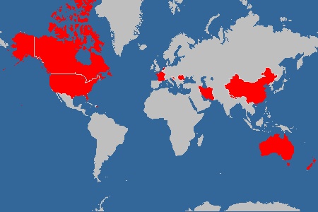Figure 1. Participants in the DARPA DMACE Challenge

2. Materials and Methods

2.1. Titanium Digital Manufacturing

Manufacturing parts in titanium often proves to be an expensive process displayed in Figure 2 and Figure 3. Notice how many extensive processes are required to modify titanium from an ore (precursor to sponge) to a final part. All of these processes drive the cost of parts made from titanium.

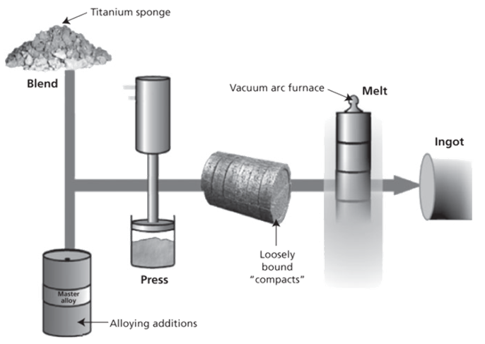Figure 2. Vacuum arc process for converting titanium into ingot [Seong]

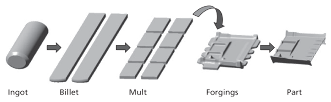Figure 3. Converting titanium ingot into a part [Seong]

Figure 4 displays emerging technologies seeking to address these processes with the goal of reducing the end cost of titanium parts. Similar evaluations may be performed for other tradition parts manufacturing.

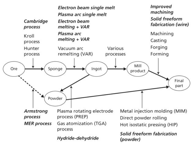Figure 4. Emerging technologies for titanium production [Seong]

Note in particular the lower path that uses relatively new additive digital manufacturing techniques to convert raw titanium powder into a final product, greatly simplifying the processing and thereby the cost. Notice the cost rising significantly in the recent decade per Figure 5.

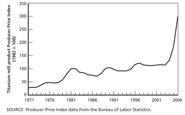Figure 5. Titanium mill products producer price index trend [Seong]

An unsolved issue is the quality of the final part produced by additive digital manufacturing (DM) methods, and this un-solved issue motivated this study.

If you needed a titanium rotor assembly for an engine, DM methods could produce such a part in mere hours in the field (potentially) directly from titanium powder, but would you put the part in your engine without any idea when the part will fail? This study addresses this question by not only addressing aluminum, but DM in general by adding a second (non-metal) building material seeking to investigate underlying properties of the process. The Challenge includes digital manufacturing of highly complex titanium and polymer parts and asks participants to analyze the data of structural tests, correlate the input settings of the DM machine to the eventual output structural properties, and then estimate the failure of an entirely dissimilar part being given the CAD design a priori.

2.2. Titanium Spheres

Titanium Spheres were digitally manufactured using an Arcam A with an electron beam (e-beam) melting process and Ti6Al4V titanium alloy powder. During the build of the titanium spheres, two input parameters in the e-beam control were varied:

1) e-beam velocity (100, 200, and 300 mm/sec),

2) e-beam current (1.3, 1.7, and 2.1 mA).

The build direction is defined as the vertical axis at which the e-beam machine built the spheres. Furthermore, each sphere had two distinct geometric axes of symmetry, which were structurally different. The two axes of symmetry were recognizable on the sphere surface by a square grid of titanium mesh or a hexagonal grid of titanium mesh along the diameter of the sphere.

For the Challenge, the build direction was aligned through the sphere diameter along one set of the square grids. This particular set of square grids was referred to as 0° from build direction. Another set of square grids was located at 90° from the build direction. The hexagonal grids were located at 60° from the build direction. Each sphere was tested in compression to failure along one of these three axes (0°, 60°, 90°) to the build direction. During the compression tests, the maximum (or ultimate) compressive load was recorded. The average maximum load, standard deviation, and maximum load of repeated tests were summarized, along with individual and summary plots, in a single Excel data file. These files are available online at www.dmace.net for registered participants.

81 spheres were tested at 0° from the build direction, 81 spheres were tested at 90° from the build direction, and 6 spheres were tested at 60° from the build direction. This equals a total of 168 total spheres as a minimum, for which the data is available to participants for model development.

The first 9 Excel files of sphere data posted on the website were crushed at 0° from the build direction, consisting of a full factorial of the 3 beam velocities and 3 current settings with 9 repeats at each condition. This resulted in a total of 81 spheres. The second 9 Excel files of sphere data posted on the website consist of the same 9 combinations of e-beam velocities and current settings, however the spheres were tested at 90° from the build direction. Both the 0° and 90° scenarios are geometrically the same; however, the 90° scenario is perpendicular to the build direction. Additionally, a single set of 6 spheres at a single beam velocity and current were tested at 60° from the build direction.

In summary: 81 spheres were tested at 0° from the build direction, 81 spheres were tested at 90° from the build direction, and 6 spheres were tested at 60° from the build direction. This equals a total of 168 total spheres as a minimum, for which the data is available to participants for model development.

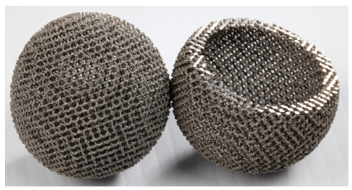Figure 6. One-piece titanium mesh spheres directly from powder

Each participant or team should use this sphere data to develop a model that will allow them to predict the maximum compressive load for various e‐beam velocities, e‐beam currents, and build directions. A final set of spheres for the Challenge finale was built at another beam velocity and current setting and tested at 60° from the build angle. This is the setting that the participants must predict based on the previous sphere data.

For the titanium spheres, models were built to predict ultimate compressive load based on the two complete factorial sets of data tested at 0° and 90° from the build angle, plus the one condition tested at 60° from the build angle. Then, contestants made predictions for the ultimate compressive load tested at 60° from the build angle with different beam velocity and current settings, which was not made known to all participants until December 3, 2010.

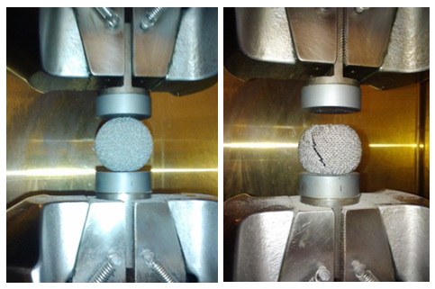Figure 7. Load-test of one-piece titanium mesh spheres

2.3. Polymer Cubes

The polymer cube problem is different from the titanium sphere problem in that initial tests were performed to establish basic material properties, and then subsequent tests evaluated structures made from the basic material.

The polymer material properties were suspected to be anisotropic and bi‐modular, so the compression and tension tests were conducted in order to establish the basic material properties of the polymer (ABS‐M30 production‐grade thermoplastic) extruded by the 3‐D printer (FORTUS 400mc). During the build of the compression and tension specimens, four processing variables were varied:

1) printer tip size (T12=0.178 mm and T16=0.254 mm),

2) machine raster angle (0° and 90°),

3) machine build angle (0° and 90°), and

4) bake time after fabrication (0 and 12 hours), referring to how long the sample remained in the printer‐oven after fabrication.

Figure 8 below provides a visual reference for the raster and build angles.

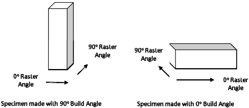Figure 8. Nomenclature for digital manufacture of polymer cubes

The second series of tests were cubes of various geometries to introduce Challenge participants to basic structural properties and to test their models. Figure 10 depicts representative cube geometries. These cubes were then tested in compression to failure, and the maximum (or ultimate) compressive loads were recorded and posted online. Based on both the material property tests and the cube tests, participants built a model to predict the ultimate compressive load of a cube design given the geometry of the cube. Similar to the spheres, the final cube geometry was made available to all participants on December 3, 2010.

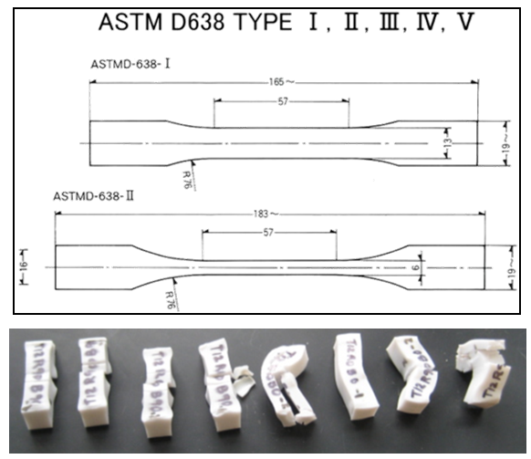Figure 9. “Dogbone” samples used to evaluate DM polymer properties

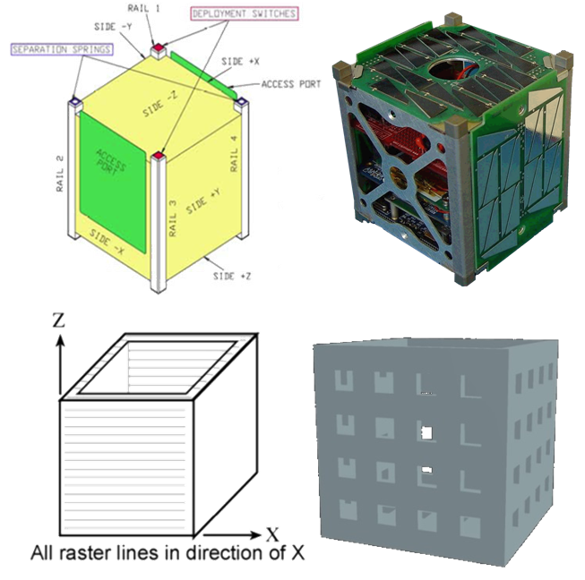Figure 10. Sample CubeSat structures

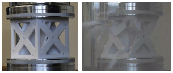Figure 11. Final contest CubeSat structure being crushed

2.4. Putting It all Together

For the DMACE Challenge, participants submitted predictions for the maximum compressive load in newtons for both the final titanium sphere configuration and the final cube configuration. Predictions and model descriptions were submitted by 1630 EST, December 6, 2010. A winner was be determined by DARPA using sample mahalanobis distance, and the winning team or individual received the $50,000 Challenge prize.

3. Results – Individual DARPA Challenge Submissions

In the paragraphs that follow, individual submissions are inserted from the original source authors listed in the acknowledgements. Only minor edits for grammar and format into this paper were made on the original submissions of the authors. All submissions to DARPA are not included in this paper, rather a sampling of several different techniques and variations of the same technique are presented here. The submissions are listed by official affiliation, while authors and participants are listed in the acknowledgements.

3.1. Submission 1: University of Missouri-Columbia

The models used for predicting maximum load for both the sphere and the cube were accomplished using neural networks. Utilizing the nftool command in Matlab, a network for each was trained using the test data to provide sample inputs and targets. Note that the inputs and targets were normalized about the maximum values for each parameter to improve network performance. The networks were then simulated under the test conditions to predict the maximum loads for both example cases.

The inputs given to the sphere network included current, velocity, and crush angle. The inputs for the cube network were tip size, raster angle, build orientation, and hours “baked.” An additional term for the aspect ratio of the loaded surface was included to make the network adaptable to various geometries. The outputs from both networks then are values between 0 and 1, which are multiplied by the respective maximum loads from each dataset to determine the final maximum load for the given case. Predicted strength for the cube is

Predicted strength for the sphere is

3.2. Submission 2: Greystones Group

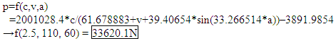
I went with a numerical analysis approach. After seeing the test data provided up to the 2nd practice question was approximately unimodal, I decided to try symbolic regression software. After seeing the data for the 3rd and final estimations it became clear that CAD or FEA software might provide better modeling for the cube. After looking at all the data and calculating the surface area of the spiral cube, I just guessed at a scaling value of the 2nd practice cube average max force. So I guess that however my brain signals were configured over the time I was looking at the data is the implicit math model for the final cube data estimate.

Math model for spheres, where force p [Newtons] is a function of current c [mA], velocity v [mm/sec] and crush angle a [degrees] (this was used for the final question estimation):

Math model for cubes, for the final question estimation:

Math model for cubes, for the 2nd practice question estimation, a area, t tip size, r raster angle, b build angle:

p = g(t,r,b,a) = a*(59.430218+38.952698*t + 7.5636129*cos(0.372657+b-0.052924275*r) / (41.201572*t*t - 0.60272503))

3.3. Submission 3: Pennsylvania State University

3.3.1. Sphere Model

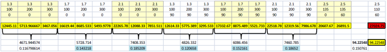
The sphere model uses the average maximum load values for the calculation average maximum force of desired conditions. First step-The standard deviation of average maximum load for currents 1.3 mA, 1.7 mA and 2.1 mA for 0 degrees of crush angle have been calculated. This calculations covers all velocity ranges (100-300 mm/sec) for corresponding current value and crushing angle. This process has been repeated for 90 degrees of crush angle. See Figure 12. Second Step- Then these calculated standard deviation values are further divided by the square of the velocity displacement of the data they have been comprised from. This would be (300-100=200). The calculated values are represented in blue boxes in the figure. Third Step-Average of all these values obtained in second step (which is calculated as 0.15076) is used to determine the standard deviation of the average maximum load for the desired conditions. This is obtained by multiplication of the average obtained value by the square of the velocity displacement for the desired conditions (135-110=25). The multiplication is due to the pattern of increase in in maximum load whenever there is a decreased velocity condition. Last Step-Having the given data and calculating the standard deviation for the average maximum load enables us to use the solver application to reach to the desired result of average maximum load of

Figure 12. Calculations of Sphere Model

3.3.2. Cube Model

The first step in cube model deals with calculating the area under compression first for a cube with no windows. Then estimated maximum stress is calculated by using the average maximum stress values. The ratio between actual load and average maximum load is calculated. (can be seen as fraction in the Figure 13) Same calculations are also carried out for the lattice cube (cube with windows) and the ratio between actual load and average maximum load is calculated. The average of these two ratios (fractions) has been calculated. After calculating spiral cube compression area and average maximum load respectively. The fraction value obtained from two previous cube calculations is used to determine the actual load for spiral cube. The final answer has been calculated as:

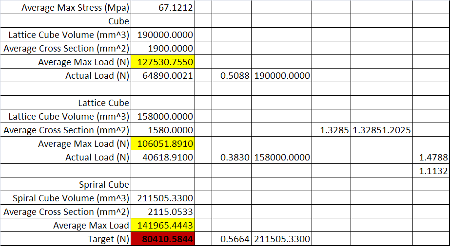Figure 13. Calculations of Cube Model

3.4. Submission 4: “Snowballs Chance”

3.4.1. Titanium Sphere Predictions

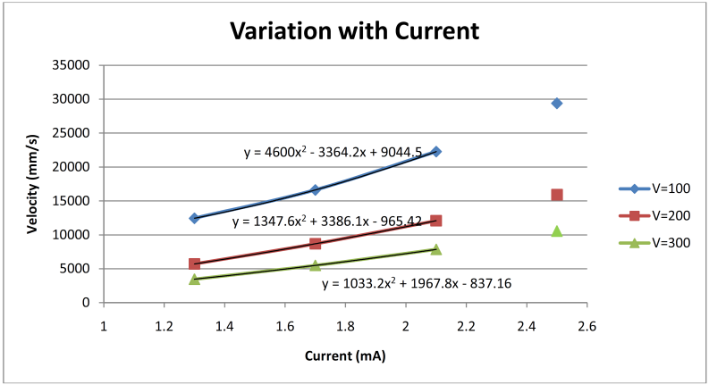
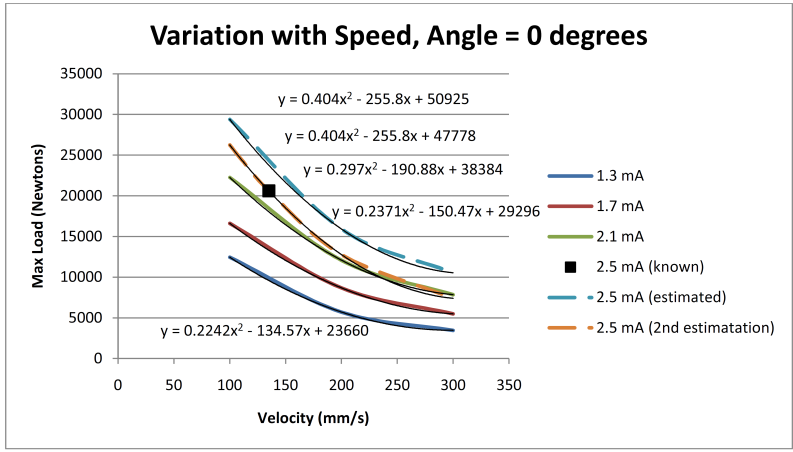
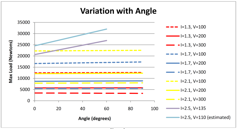
The goal of the titanium sphere predictions was to estimate the maximum compressive load that a sphere made with a current of 2.5 mA, velocity of 110 mm/s, and a crushed at an angle of 60 degrees could sustain. There is no given data for a velocity of 110 mm/s, but there is data for velocities at 100, 200, and 300 at angles of 0 and 90 degrees with currents of 1.3, 1.7, and 2.1 mA. There is also data for current at 2.5 mA and 135 mm/s and an angle of 60 degrees. The first step taken in the modeling process was to predict what the curve for a variation with speed chart would look like. This was accomplished by using Figure 14 and extrapolating to determine how much the maximum load varies with current. The right set of data points in Figure 14 are the estimated data points.

Figure 14. Sphere data extrapolation

This data was then plotted on a variation with speed curve for a crush angle of 0 degrees, as shown in Figure 15. This yielded the quadratic equation: y=0.404x2 – 255.8x + 50925, shown by the blue dashed line in Figure 15. However, this did not match the known data, which can be seen because the blue dashed line does not intersect the known data point. Therefore, a C value in the quadratic equation was solved for so that the estimated curve fits the known data, which is shown by the orange dashed line in Figure 15. Using the new equation, y=0.404x2 – 255.8x + 47778, the maximum load at a velocity of 110 mm/s was solved for. It should be noted that this model is probably not accurate for higher velocities because of insufficient data in that range.

Figure 15. Sphere data extrapolation

Lastly, the strength at a crush angle of 60 degrees was solved for. Figure 16 shows how the maximum load usually varies with the crush angle. Typically, with an angle of 0 or 90 degrees there is not much variation. However, as shown by the purple curve (I=2.5, V=135) there is variation with a crush angle of 60 degrees.

Figure 16. Sphere data extrapolation

Therefore, to estimate what the strength would be for a crush angle of 60 with I=2.5 mA and V=110 mm/s the percentage increase from 0 to 60 degrees was calculated for I=2.5 mA and V =135 and this data was applied to V=110 mm/s. The percentage increase was 30.493%, so the predicted strength for I= 2.5 mA, V=110 mm/s, and a crush angle of 60 degrees is

3.4.2. Cubic Predictions

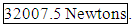
The goal for the cubic predictions was to model the maximum load that a digitally manufactured cube could withstand. In order to accomplish this, the maximum load on a cube with solid outer walls was known, as well as the maximum load for a cube with lattice outer walls. The unknown was a cube built as in Figure 17.

Figure 17. Unknown Cube configuration

The method that was used to solve for the maximum compressive load involved a finite element model. Since the model is concerned with compressive fracture, the maximum compressive principle stress was used for calculations. Figure 18 shows the finite element models used for the two known samples.

Figure 18. Known cube configurations

These samples had a nominal load of 20,000 applied at the top, and the maximum compressive loads from the finite element model were nominally -8.42 for the solid walled cube and -13.9 for the lattice cube structure. This means that the solid walled structure would only see 60% of the stress of the lattice structure. This also matches closely with the given data, where the average maximum load for the lattice structure was 62% than the maximum load for the solid walled structure.

Figure 19 shows the finite element model for the final test specimen. In this case, the maximum compressive principle stress was nominally -12.3. This is 68% the strength of the solid walled structure and 113% the strength of the lattice structure. Therefore, the predicted maximum load for the final configuration would be either 44,420 N if going off of the solid walled cube or 45,900 N if going off of the lattice structure. The best estimate the model will give is an average of these two values,

Figure 19. Final test specimen

3.5. Submission 5: Embry-Riddle & Harvard Cavanaughs

The DARPA DMACE Challenge seeks to determine if it is possible to predict the strength of a structure constructed via rapid prototyping methods. This contest will select the participant group with the closest estimation to two test samples as a winner, provided that documentation of the method used in the estimation is provided. This document describes the method used by “Team Cavanaugh" in fulfillment of that requirement.

3.5.1. Sphere Challenge

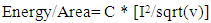
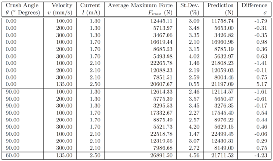
The sphere challenge tested a complicated spherical shape with 6-fold symmetry made of a titanium alloy with the Arcam A2 additive manufacturing device. This device uses an electron beam to melt a titanium alloy powder, thus fusing together neighboring pieces of the powder into a solid structure. The input parameters to the machine included the speed at which the beam was moved across the material, v, and the current of the electron beam, I. Spheres created by this system were then tested for strength by crushing the sphere at in a direction relative to the build angle, (either 0° or 90°). For each combination of input parameters and crush angle, a sample of ten different spheres was generated and tested.

The Model: The goal of this model is to be able to predict the strength of an sphere created with an arbitrary set of input parameters and crush angles. Here, the strength of a sphere is defined as the average maximum amount of force, F_max, that a sphere can withstand before complete failure. A decision was made to separate the data based on crush angle in the event that there was some angular dependency. A prediction for an arbitrary angle and input parameters, P(v,I,θ) would then be calculated by combining the prediction for the tested angles according to the following way:

(1)

Such a prediction would only take into account differences in the objects strength due to the underlying materials strength. It would then be necessary to scale such a prediction for an arbitrary angle to account for the additional changes in strength due to the actual shape of the structure. In this case, since the sphere has 6-fold symmetry, it is expected that some difference in strength will be located about a 45 crush angle. However, no tests are made in this configuration. Therefore, any final prediction would include a material strength adjustment as shown in equation 1 that has been shifted up or down to pass through a given test point for a non trivial configuration (that is, an angle not equal to 0 or 90). Since the general principal behind this manufacturing process is similar to welding, it was decided that the strength should be proportional to the amount of energy applied over a given area. The power delivered by the electron beam is proportional to I²R, where R is some arbitrary system resistance. This power is delivered over a longitudinal area per unit time specified by v. The transverse area is given by the beam spot size, which is proportional top I. Therefore, the resulting formula for applied energy per area is given as

(2)

where C is an arbitrary constant of the system.

A decision was made to t the provided data for a statistical approach to the problem. It is expected that the actual behavior would be something like F_max ln(Energy/Area) in general. However, since the parameter space that we are looking at only covers a portions of this curve, we can safely approximate the behavior with a second order polynomial. The Energy Area values obtained from the data are summarized in Table 1. These values were t separately for each of the compression angles. A plot of the data points is given in figure 2. An uncertainty of 5% was assumed for each of the machine input parameters, resulting in roughly a 12% uncertainty in the Energy Area parameter. The resulting t parameters are given in Table 2.

Table 1

Table 1 displays the sphere test data. Predicted values are shown using the fit values found in Table 2. Note that a separate fit is not done for each test case and that the actual value for a test point is included in creating the estimation for that point. The 60° case presented here only accounts for material differences in that configuration. The prediction presented does not take into account differences due to the 6-fold symmetry of the structure.

Table 2 displays the resulting fit parameters for F_max=P₀ + P₁(Energy/Area) + P₂(Energy/Area)². Note that the fit for 60° is an estimation obtained from combining the _t results from the 0° and 90° cases and shifting that result to pass through the only 60° test point.

Table 2

Figure 20 contains a plot of the maximum force sustained, F_max, by the test spheres as a function of the Energy/Area for each of the crush angles. The black curves illustrate the result of the second order polynomial fit. The dashed curve illustrates the t obtained from the 0° and 90° cases combined and shifted to pass through the only 60° test point. This estimation is done to both accounts for material strength at 60° and for the structural differences in the 6-fold symmetry structure at this angle.

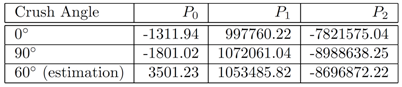
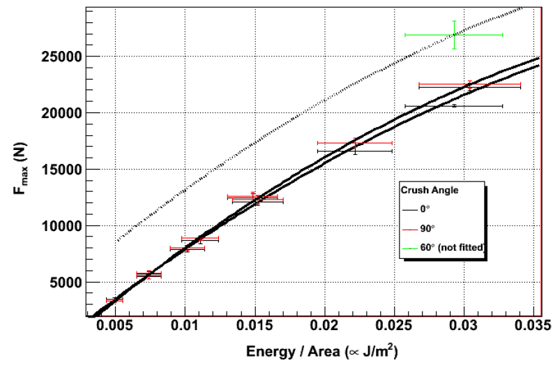Figure 20. Maximum force sustained versus energy/area

The Challenge Prediction

The final challenge asks for a prediction of the maximum force, F_max, that a sphere of this design can withstand with the machine parameters I=2:5mA and v=110 mm/s and with a crush angle of The prediction for this set of parameters is

Sphere Summary

While this statistical method provides a means to predict the strength of this unique spherical structure, this exercise does not actually examine the resulting properties of the material formed. A more thorough test would have generated bar samples for material strength tests, as done in the other part of the challenge. Very little is known about the underlying structure of the material. It would have been instructive to have samples crusted at 45°.

[1] 3.5.2 Prototype Method 2 - Thermoplastic

The second challenge tested a different manufacturing technique which involved creating various sample geometries, and cube-structures in a FORTUS 400mc thermoplastic 3-d printer with ABS-M30 thermoplastic. The manufacturing process involves a variable width nozzle that extrudes the thermoplastic material in layers. The final geometry to be tested was one roughly the size of a cube- satellite. Cube satellites are purpose built for a multitude of missions but they share the same external dimensions. Having an ability to build and predict performance of various structural designs would be highly desirable. Compression and tensile tests were performed on the thermoplastic samples to demonstrate the material properties of the various manufacturing orientations. Each set of samples differed by extrusion diameter, raster angle (the direction at which the nozzle moved while extruding the thermoplastic in the oven), and by build angle (the direction between the longitudinal axis of the part and the oven floor). Half of the samples were heat cured for 12 hours prior to test. Three cube structures were then produced with various open and closed wall designs, similar to many weight saving techniques used in aerospace structures. The first two were sample designs and the third was the challenge test subject. 2.1 The Model This method of manufacturing seems to have much higher repeatability as compared to the Arcam A2 machine. The test structure is a five sided box with solid sides. This structure can withstand 64890 ± 779.8867 N before failure. The contest asks us to predict a structure that has cutouts. The solid wall box can be estimated as being comprised of many adjacent columns. When the cutouts are made, the number of effective columns is reduced.

In the test cutout box, the effective column count is reduced by 40% when four columns of 10 mm cutouts are made per side in the 100 mm per side box, the resulting strength should be reduced by 40%. This thinking leads to a prediction for this test structure of a maximum force of 38934 ± 467.93 N which is well within the agreement of the actual value which is 40616.91 ± 885.19 N. Note that the estimation is off by only -1.9.

The Challenge Problem

The challenge problem provides for a more complicated problem that the simple cutout challenge problem. The structure now has no bottom, has substantial cutouts of the four sides (with cross members) and has an inner spiral which serves to give a non uniform support to the walls. This structure is substantially different from the other two structures because it does not have any bottom. As such, it can be roughly modeled as four corner columns held in a configuration by the cross members. The box is loosely prevented from caving in by the spiral structure, although it is not simple to perform this calculation without advanced simulation software. The estimation therefore will seek to pull the entire strength of the structure from the four corner beams. Each corner beam is approximately 10mm on each side and 5mm thick. This Following the adjacent column model described previously, this would result in a total of 80mm of 5mm thick columns for the wall of the structure. The center of the spiral provides an additional 5mm by 5mm column, for a total of 85mm of effective 5mm column. The test box had effectively 400mm of 5mm column. Therefore, neglecting the absence of a bottom, this final challenge box should capable of support a force of 85mm/400mm X 64890.00N = This estimation does not account for the fact that the structure is more likely to fail after rotating about Z, whereas the original test box did not express a rotational preference as a failure mode.

Thermoplastic Summary

This statistical method relied on more consistent sample sets; however each sample set only contained only two data points. Additional repetitions of each sample set would have improved the robustness of the model. More complex cube-sat geometries would require different lab tests to be conducted to test the shear-interface between multiple layers of thermoplastic.

3.6. Submission 6: North Carolina State A&T University

A general regression neural network (GRNN) was used to model both the sphere and the cube problems. Data from the previous practice problem was utilized as past history to develop the models. The GRNN is a statistical technique that estimates the most probable curve to fit a collection of points by optimizing the choice of a set of model parameters. It consists of four layers:

1. Input Buffer

2. Gaussian Displacement Layer

3. Summation/Divison Layer

4. Output Layer

The input buffer distributes the activity patterns of the input to the neurons in the Gaussian displacement layer. The computation of the Gaussian displacement layer is governed by the following equations.

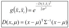(3)

A Gaussian matrix is formed to represent the entire system such that a set of weights can found to represent the relationship between the Gaussian transformation of the input space and the target output. Weights are obtained using a pseudo-inverse.

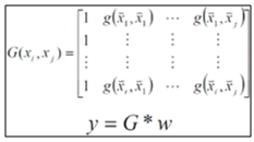(4)

Table 3

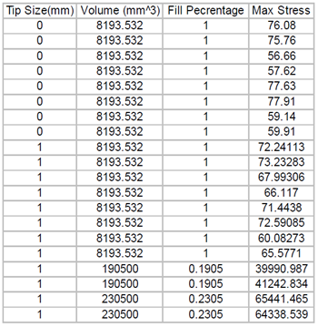
3.6.1. Cube Problem Data Set

The cube problem data set was formed only from the data given for the compressive load of the previous cubes and only cubes with a 0 degree raster angle. The features in the data set consisted of the type of tip size used, volume of material that made up the cube, and the estimated percentage of material missing from the with respect to its overall volume. To get the fill percentage we estimated the volumes of the cutouts within the box such as the inner triangles in the final block. Max Stress served as the output for the model. (Example below)

Final Cube Parameters Used

Tip Size: 1

Volume: 205250 mm

Fill Pct: 0.20520

Predicted strength is

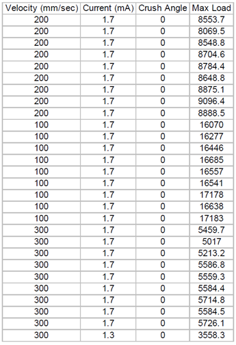
3.6.2. Sphere Problem Data Set

The sphere problem data set was formed from all of the past data given in the practice problems. The features in the data set consisted of the velocity, current, and crush angle. (Example below)

Table 4

Predicted strength is

3.7. Submission 7: Auburn University

3.7.1. Modeling of Maximum Compressive Loads for Titanium Spheres

Machine: Arcam A2 (electron beam melting process) Parameters

v = e-beam velocity (100, 200, and 300 mm/sec),

I = e-beam current (1.3, 1.7, and 2.1 mA).

E = e-beam energy

Material: Ti6Al4V titanium alloy powder, Tensile Strength [Titanium Information Group]: min 897 MPa, typical 1000 MPa Tensile Strength [Arcam data sheet]: req, 860 Mpa, 930 Mpa, typical 1020 Mpa. Elastic Modulus [Titanium Information Group]: 114 GPa, Modulus of Elasticity [Arcam data sheet]: 120 Gpa.

Angle between build direction and compression testing direction: a (0, 60, and 90 degrees). Sphere Dimensions: The outer diameter is approximately 40mm and inner diameter is approximately 30mm.

Model

We denote by F the maximum compressive load.

After analyzing the data, we have the following relations between the involved parameters. Provided that the angle between build direction and compression testing direction is fixed, E-beam velocity (v) is proportional to ln F and also e-beam current (I) is proportional to ln F. So, we have a plane as the surface of the function which gives ln F in function of v and I:

(5)

where A, B, and C are constants to be determined using the data. Since, we are assuming linear relations we will take the information of the three most accurate points (with the smallest standard deviation) to find A, B, C, and D.

he points are: P1 (1.3, 300, 3467.06), P2 (2.5, 135, 20607.67) and P3 (1.3, 200, 5713.97) or with ln F we have P1 (1.3, 300, 8.151061), P2 (2.1, 300, 8.968461) and P3 (1.3, 200, 8.650669). With the calculated values for the coefficients, the corresponding mathematical model for F will be:

11503882298164500 I - 56250860065783 v - 11258999068426240 (ln F) = -93692999237806510

or

ln F = (11503882298164500 I - 56250860065783 v + 93692999237806510) / 11258999068426240

Then, we correct for the testing angle with the factor

(6)

where E is a constant to be found with the testing data at angle 60 degrees. The value for E is -0.05. So, the model is

F=[1+(0.010269(2a)/Pi-0.05Sin(2a))]

*exp[(115e1403882298164500I¬56250860065783v+93692999237806510)/ 11258999068426240]

Estimation (in newtons) of the maximum compressive load of a sphere that is digitally manufactured using the following setting:

Current = 2.5mA Velocity = 110 mm/sec Crush Angle = 60 degrees

3.7.2. Modeling of Maximum Compressive Loads for Polymer Cubes

Machine: FORTUS 400mc (3D printer) Parameters

• Printer tip size (T12=0.178 mm and T16=0.254 mm)

• Machine raster angle: R (0° and 90°)

• Machine build angle: B (0° and 90°)

• Bake time after fabrication: t_c (0 and 12 hours)

Material: ABS-M30 production-grade thermoplastic [ABS-M30] Tensile Strength: 36 MPa Tensile Modulus: 2413 MPa Flexural Strength: 61 MPa Flexural Modulus: 2317 Mpa. Compression test specimen geometry: square prism of nominal dimension of 12.7 mm x 12.7 mm x 50.8 mm.

MODEL

We denote by F the maximum compressive load. According to the experimental data for maximum stress, the build angle and raster angle affect it as follows: It is ordered from higher to lower R0B0, R90B0, R0B90, and R90B90. Smaller print tip size gives higher maximum stress only for the case R0B0.

For testing failure we have two options: 1) Compression failure (depends only on critical cross-section area) and 2) Buckling failure (depends directly on the Inertia of the critical cross-section area) by Euler buckling equation. Since the manufacturing process is process is by printing (depositing material), the arrangement of material is layer by layer of a given thickness and the adhesion of one layer against the neighbor layers is the most relevant. So, we will correlate the maximum compressive load with both the smallest critical cross section area (A₁) and the lowest Inertia (I_x and I_y) of a critical cross-section area A₂.

(7)

With the data we find p and q. Estimation (in newtons) of the maximum compressive load of a spiral-cubic structure built with tip size 16 (0.254mm) at raster angle as depicted in 'SpiralWebWindowCube_V2_dwg.pdf' and a build angle along the Z axis that has these dimensions: 100 mm x 100 mm x 100 mm (outside dimension), Wall thickness 5mm.

The top and bottom sides are open while the remaining four sides have an 'X'-shaped structure. The compressive load will be applied along the Z-axis; that is, in line with the axis of the spiral inset

3.8. Submission 8: Isakson Engineering

3.8.1. The Sphere

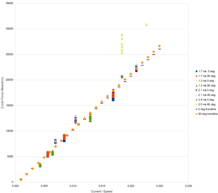
The first realization that occurred to me was that the strength of the material is likely a function of the energy put into a given point of the sphere. The rational for this is that the material with more energy put into it will melt together better. So the higher the beam current and the slower the scan, the more energy added and the stronger the material. So I reorganized the data to show the yield strength verses the quantity current/speed. Additionally, however, I expected some leveling off of the strength at higher energy levels as the material will at some point reach the ultimate strength of the raw material completely melted together. I therefore tried to match the data to a sigmoid curve. However, no set of parameters for this seemed to be a good fit. My conclusion is that we are still some distance from the ultimate yield strength (and possibly a sharper inflection then a sigmoid is needed). More tests would have to be performed to determine what the ultimate strength while maintaining good manufacturing tolerances. I therefore fitted the data to a straight line and found a reasonable fit. In Figure 21, you can see the results of this plot. As part of this plot you can see separate trend lines for both the 0 degree crush angle and the 90 degree crush angle. It can be seen that the results indicate slightly higher crush strength at 90 degrees, particularly at higher input energy levels. As will be seen later, this difference is small compared to another problem with the data. This plot also suggests a small change at higher current levels as well. The plot suggests that the higher currents cause a higher strength in the mid energy levels which might decline again at higher levels. This would require the fitting of a curve to fit this, but I do not believe there is sufficient statistics to justify this. Also, a straight line could be fit to just the 2.1 ma (or 2.1 ma and 2.5 ma), 0 degree data (it would change little if the 90 degree data was included as well). However, such fitting would only change the final result a little bit.

Figure 21. Data fit to straight line

Even a weighted fit changes only results in minor changes as the 0.021 current/speed data would tend to dominate and it is close to the trend lines. In the end, I chose to use the 0 degree trend line as the basis for the prediction, as 0 degrees was a given set of data points that was experimentally determined. I used that trend line to predict the force needed for a 0 degree failure for a energy of 0.02273 (2.5 ma and 110 mm/sec). From there I used the ratio of the mean 60 degree failure to the mean 0 degree failure at 2.5 ma and 135 mm/sec to project the failure level at the final desired solution level. This use of the ratio assumes that the failure level for 60 degrees would also fit a straight line to approximates zero (it is not exactly that, but close) to be valid, but I do not think that is a bad assumption.

The final result was (which I consider the best estimate with the available data). The previous explanations could certainly justify increasing or decreasing the result a little bit, but these errors are minor compared to the last step of the procedure outlined.

While the standard deviation (SD) at low energy levels tended to be in the 4% range, as the data moved to higher energy levels the SD fell to around 1.5%. The regression line would have been even better. The limited 2.5 ma 0 degree data was less than 0.4%. However, when the 60 degree data was presented, the SD rose to 5%. I would have thought this was manufacturing out of control, except the 0 degree data came from the same batch and it was highly controlled. As a consequence, this large standard deviation is the largest source of error (by far) in the final result. I would look for a different method of generating this final step, but the data at 60 degrees is very limited and this appears to be the best procedure available.

While I do not know what is causing this large SD in the 60 degree crushing tests, I would expect this same problem to exist in the final spheres as well which will give a lower sample Mahalanobis distance.

3.8.2. The Cube

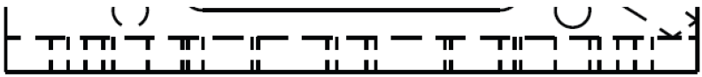
To determine the crushing force for the cubes, I split the cube into three parts and two types of faces (a total of 6 areas to determine). The three parts are the corners, the X portion on the face, and the spiral. The two faces are the face parallel to the raster scan and the face perpendicular to the raster scan (it is a little more complicated for the spiral, but the idea is the same). For each case, there is two of each part, so the force is multiplied by two. To start with, I should say that while I have some models of how the failures should be occurring, I have found that much of the data does not agree with my (mental) models. As I consequence, I must yield to the data and much of my conclusions as to the final force is based on the data tests result more than what I think should have (but obviously did not) happened. So if my explanations seem to leave a little to be desired, my apologies. I will tell you how I calculated the results I provide. One of the first assumptions that I am making is about the (mounting) holes in the sides of the cubes. They are all located in areas that have a significant polymer around them. As a consequence, I do not believe they will lead to a failure and therefore I am ignoring them. However, confirmation of this would be one advantage to finite element analysis, which I did not do.

The Corners

Figure 22. The corners

It is my belief that the side parallel to the raster scan fails at a lower level than the portion perpendicular to the scan. This is shown in the data as well as a model about how a wall fails. The one exception here is that each wall is very short and does not completely qualify. However I will still use the same model here (for lack of a better model that would require finite element analysis that I do not have access to and did not set up in advance as the practice questions were simpler). The only question is how I treat the corner (the 5 mm by 5 mm area). I will treat it as if the entire corner is on the stronger side.

This corner is roughly 9 mm on each side with 5 mm thick walls. This gives an area of 45 sq mm on the strong side and 20 sq mm on the weaker side. In addition there are four corners, so these areas are multiplied by four. The first side gives way at a strain of 0.01252 mm/mm and a pressure of 30.59 MPa. The second side gives way at a strain of 0.01849 mm/mm and a pressure of 66.43 MPa.

Applying this data would give a force plot similar to Figure 23.

Figure 23. The corners

Note that I have shown a failure as total and a drop in force. The real plots do not tend to show a sudden drop always. We will see if this makes a difference.

The X Portion

This can be analyzed in a similar manner to the corners, except there are new types of stresses. (Please note that I accidently placed this picture in upside down from the conventional thinking. The place where the pressure is applied (the + z axis) is at the bottom. This however makes no difference in the results, so I have no time for replacing this picture).The top and bottom are about 9 mm wide and the 45 degree cross bars are about 18 mm wide. As the force is applied at an angle (45 degrees) to the raster scan, there are more direct shear forces at play. This is particularly significant since the material is anisotropic.

Additionally, the top and bottom horizontal bars are put in tension. On one face this is a particularly strong bar and on the other a weak bar. At this time I am not giving credit to the forces applied from the corners to help take tension off the bars as these forces would add to the corner failures to some extent. On the parallel to raster scan the top bar is the strong T16R0B0 configuration with a tensile strength of 62.77 MPa. This is what I normally consider the weaker of the two wall however (the side I expect to fail first). The other side has a T16R90B0 configuration with a tensile strength of 50.05 MPa. This gives the forces at failure of 2824.5 Newtons and 2252.3 Newtons for each single bar. Meanwhile, the pressure on the diagonal is the vertical pressure divided by the cosine of 45 degrees. And the pressure in tension on the top and bottom bars is (by vector addition) equal to twice vertical pressure (since the wide of the horizontal bar is half the 45s – and therefore twice the pressure to equal the vertical force). The parallel side then fails at a pressure of 21.63 MPa (A strain of 0.00602) (the pressure on the diagonal causing failure on the weaker side) and the perpendicular side would fail at 25.03 MPa (A strain of 0.00697) in tension on the top bar. This all ignores the shear component, but I suspect that is not a big deal right now. This gives a stress-strain plot of Figure 25.

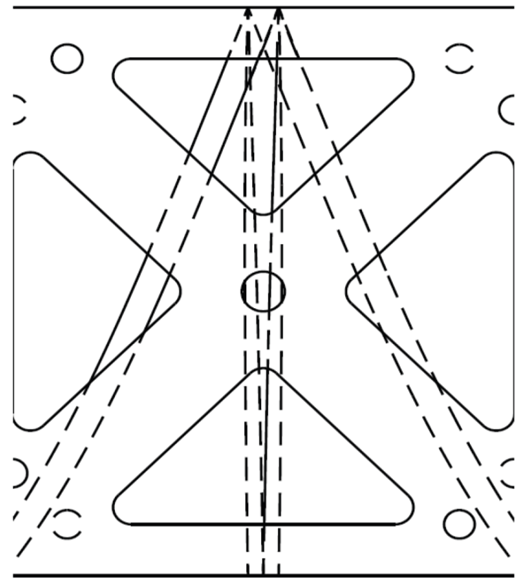Figure 24. The X-portion

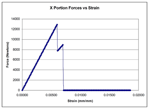Figure 25. The X-portion

I suspect I have underestimated the forces to some extent, but this is my best organized guess at this point.

The Spiral

(I cannot find a good picture to put in here, but I think you understand the portion I mean in the center of the cube). This item is best modeled using finite element analysis (more so than the other portions). However I give it a shot here. Again I am going to ignore the shear forces and the chances for delaminating of the layers, since my models of the material are too crude for a good analysis. The spiral is a constant area from top to bottom (225 sq mm for each of the four arms (including half the center shaft that does cause a little overlap). The angle of the pressure is perpendicular at the center and 30 degrees at the outside. This increases the pressure on the outside. Additionally the cross section in the plane of the force is smaller. I will again assume a strong side and a weak side (though this is somewhat confused by the rotation). Failure is assumed to start at the outside (with its higher pressure because of the angle) and will move to the center at constant force (increasing pressure) until the failure at the center. The result is Figure 26.

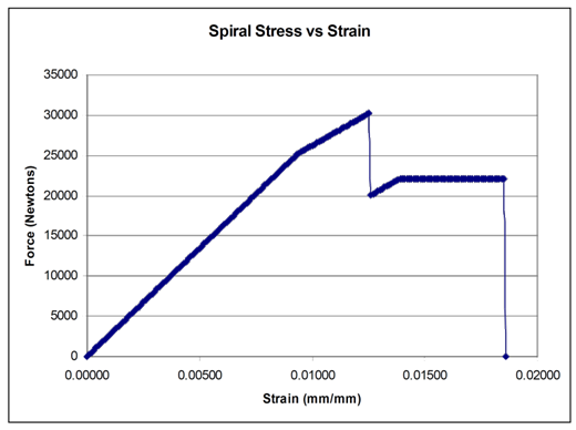Figure 26. The spiral

The Final Result

Summing these all together you get is displayed in Figure 27 with a maximum force of

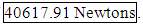
Figure 27. The final result

3.9. Submission 9: University of California, Santa Barbara

3.9.1. Sphere Crushing Model

The prediction of the sphere crushing load was obtained principally from finite element calculations. To this end, a script was used to generate a model of 1/8^th of the sphere, starting from a single unit cell of the lattice structure. The strut length was taken to be 1.08 mm and the inner and outer sphere radii were 30 and 40 mm, respectively. Several different values of strut diameter were used. The mechanical response of the Ti6Al4V alloy was represented by a bilinear material model (Young’s modulus E=120GPa, yield strength σ_y=950MPa, tangent modulus in the plastic domain E_t=0.012E, and Poisson’s ratio ν=0.3). The cut faces of the sphere section were constrained to in‐plane motion as the sphere was crushed by an analytically rigid surface.

The key unknown in the challenge is the strut diameter and its variation with deposition conditions. This was inferred from comparisons of the finite element results with the experimental measurements for crushing parallel to the build direction. The results suggest that the key parameter controlling the strut diameter and the sphere crushing load is Ω = I^1.31/V where I is the current and V the velocity of the electron beam. Finite element calculations were then performed for sphere loading at 60° to the build direction using the pertinent values of strut diameters in order to infer the sphere failure load.

3.9.2. Cube Crushing Model

1. Stress strain data for compressive samples were converted to true stress vs. plastic strain. 2. The ratio of flow stress in the R-B90 and R90B0 to the R0B0 direction was calculated from representative curves and used to define a Hill criterion yield surface with the plastic strain hardening data from the R0B0 direction. 3. The elastic modulus for each orientation was measured at stresses from 10-25 MPa and used to define orthotropic elasticity. 4. The solid walled cube was simulated using these parameters. It was assumed that the wall thickness was slightly different from the specification due to the printing process. The wall thickness in the model was adjusted to match the initial measured stiffness of the structure (adjusted wall thickness = 4.68 mm). 5. The spiral web cube was simulated (in Abaqus/EXPLICIT) assuming a 4.68 mm wall and web thickness. 6. Structural collapse was assumed to occur when the tensile failure strength in a given composite direction (20.7 MPa between build planes, 50.1 MPa between raster lines in the build plane, 62.5 MPa along the raster lines) was exceeded. The load at this point was reported as the peak load of the structure.

3.10. Submission 10: North Carolina State University

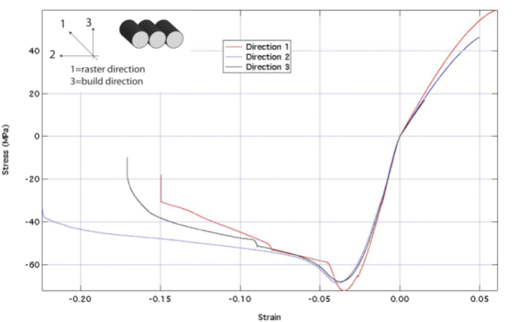
3.10.1. Cube Challenge (See Figure 28)

Model of Buckling Load Factor (BLF) and Applied Load: Calculate BLFs using computation methods (x), employ applied load (y), compute FS bias (z), then F(x,y,z)=x*y*z. Vary material properties to fit data. Resulting

Figure 28. Cube geometries

3.10.2. Sphere Challenge

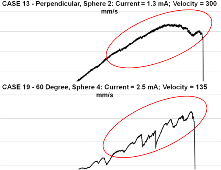Figure 29. Sphere crushing behavior

No model required for the sphere’s final challenge! Crunching behavior exhibited! The reason why the load is so high is because of the organized successive collapse at 60 degrees. Independence from build parameters! Hence the maximum load for the sphere is equal for all parameters when tested at 60 degrees. Although I have no model for the final challenge I built several models for the practice rounds (I won the first practice run doing so), resulting in a best estimator is mean provided by 60 Degrees data.

3.11. Submission 11: Washington University in St. Louis

3.11.1. Titanium Sphere

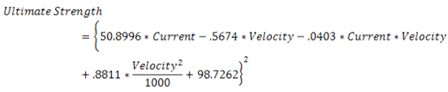
With the amount of data presented for the Titanium Sphere we were confident an accurate mathematical model could be found based solely on statistical analysis. Our program of choice to perform this analysis was the free software ‘R’. We began by importing all 9 runs for the first 17 sets of data provided on the sphere. Variables were designated as Current, Velocity, and Angle. We then used R to perform a linear regression on the data including all the cross terms of the variables. An analysis of variance showed that the only significant variables were Current, Velocity and Current*Velocity. However, the coefficients generated for these variables did not provide an accurate model. Looking at residual plots of the variables, it appeared a nonlinearity was not being accounted for in Velocity and possibly Current. We performed the analysis again this time including Velocity^2 and Current^2 terms and their crosses. Velocity^2 was divided by 1000 to make its magnitude more comparable to the other terms. An analysis of variance showed the significant terms to be Current, Velocity, Current*Velocity, Velocity^2/1000 and to a less extent Current^2. We dropped Current^2 and were left with four terms. To reduce the range of the Ultimate Stress to a smaller range we changed our model to solve for the square root of the ultimate strength. When data set 18 became available we checked our model against the given value and were satisfied with the results. We then included all 18 sets of data and solved for the coefficients again. This left us with the following equation:

After data on the spheres crushed at 60˚ became available, we again tested our model. It gave an error of about 12% so we decided to go back and try to find a dependence on angle. Repeating the analysis, however, did not return any new significant variables. The dependence on Current^2 increased slightly so we included it in our final model:

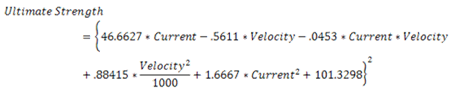Using this approximation the predicted value for a Sphere constructed at 2.5mA, 110mm/sec and crushed at an angle of 60° is

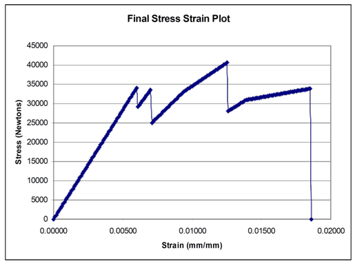
3.11.2. Polymer Cube

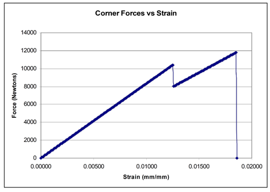
The shape of the stress-strain curve exhibits an unusual behavior. It increases fairly linearly until it reaches its ultimate strength, common for brittle materials. Thereafter, the stress decreased with increasing strain until it could no longer support any loading. This behavior can either be attributed to strain-weakening in the material or is an artifact of the compression test method used (the material failed at the peak and the crumbled structure continued to offer some support). We concluded that the material is primarily brittle and failure coincides with the ultimate strength.

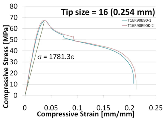Figure 30. Cube stress-strain

The data provided for the T16 material samples in compression was used to obtain an effective modulus of elasticity of the material. The averaged ultimate strength of the two T16R90B90 samples and their averaged associated strain produced the following line whose slope was extracted as the modulus of elasticity for all our work. This modulus is 1781.3 MPa.

Initially, hand calculations were performed on the Practice 1 cube structure to get a feel for the behavior of the geometry. This back-of-the-envelope analysis first modeled a wall of the cube as a thin plate to find its buckling strength. The ends of the plate were considered to be simply supported and the sides clamped. In addition, we calculated the short beam buckling of the cube minus the bottom. Ultimately, the final structure of the cube was too complex to continue this simple analysis.

From there we move to finite element analysis in Stress-Check. The material was chosen to be a perfectly elastic material to keep the analysis linear. Using a compressive loading of -1 on the top surface, we could find the maximum local stress concentration. This value or the average of the stress in a particular area could be used to find failure of the structure. Considering the setup for the compression test, we again took another approach. We imposed a 1 mm downward displacement on the top surface of the cube. We had already decided that the corners and the central axis of the spiral were the primary load carriers, so we took the maximum principle strain on a column which was found to be .02004 mm/mm. Since, the analysis was linear, it was straightforward to come up with a linear relationship between this strain and the stress on the top surface of the cube (5.878 MPa) combined with the strain at failure of our material, we got the following relationship and result of

3.12. Submission 12: Lamar University

3.12.1. Sphere Model

A kriging model based on the 20 experiment points (Average Max Load) was constructed. Pattern search was used to find a suitable set of parameters. The generated kriging model was evaluated in a MATLAB .m file containing Matlab script. The predicted strength for 60 degree, .5mA and 110 speed is

3.12.2. Cube Model

Material Model: Linear elastic orthotropic structural material. The young’s modulus was estimated based on the cube compression test results. The strength along the raster direction is the highest (75~77 MPa), while the strength representing the bonding strength between layers are the weakest (57~59 MP), the bonding strength between raster is slightly better (61~63 MP). Since the loading is along the weakest direction, it is expected that the failure most likely to be caused by the stress along the loading direction exceed the ultimate strength of the material. A FE simulation model was built in Ansys with the following material properties:

EX = 2.34 E9; EY = 1.86E9; EZ =1.97E9;

Rho_xy = Rho_yz = Rho_xz = 0.48.

GXY = 6.65E8; GYZ = 7.85E8; GXZ = 6.28E8.

The estimated maximum load is

3.13. Submission 13: Team PAM (UC Irvine, Rapidtech, CalRAM)

ASIDE: This is a note from the authors. Submission 13 has been substantially modified in form-only, but unaltered in content. The form was modified to accommodate comments by peer reviewers regarding the unwieldy presentation of regression formulas and results. These items have been reformatted by the authors merely for athletics.

3.13.1. Synopsis and Problem Statement

The DMACE Challenge has been to determine the maximum compressive loads that can be supported by two structures manufactured by direct digital manufacturing methods. The structures were a mesh sphere manufactured by the Arcam electron beam melting process using Ti 6Al 4V and a cube with an internal structure manufactured by the Fortus 400mc 3D Printer extruded polymer process using ABS-M30. To address this challenge, a team was assembled comprising Professor Lorenzo Valdevit’s research group and others from the University of California, Irvine, Rapidtech – the leading educational organizational group for freeform fabrication, and CalRAM – the leading vendor for titanium parts built by the Arcam process in the US.

3.13.2. Overview of Modeling Approach

The two structures were addressed using different approaches. In the case of the sphere, the team felt that the dimensions of the sphere’s detailed structure were too close to the resolution of the build technique to enable the spheres to be reliably modeled with a lattice model using known Ti 6Al 4V handbook properties; additionally, the posted data showed relatively minor anisotropy. Therefore a numerical approach based solely on provided measurements was adopted. In the case of the cube, a finite element model of the final challenge structure was built and necessary choices were made about material response in order to have a model that would run within the available time for the challenge.

These approaches are described below.

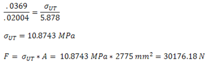
3.13.3. ABS Cube

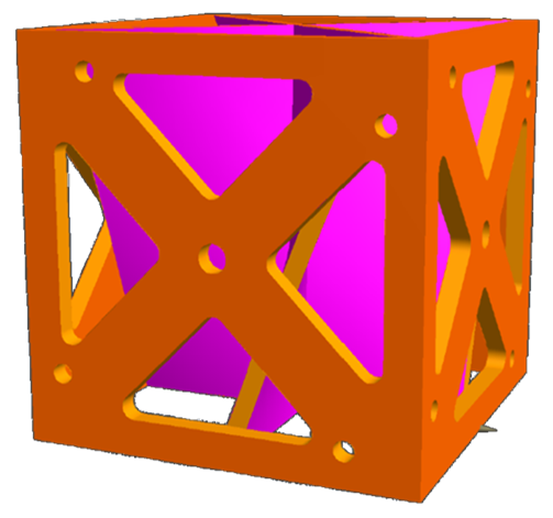
Cube prediction methodology [Lorenzo Valdevit, valdevit@uci.edu] Tensile and compressive test data were provided for a number of samples, along three different orientations: raster direction (1), build direction (3) and the direction normal to 1 and 3 (2). The results were very reproducible, with minimal scatter. Representative stress-strain curves for a tip diameter of 0.254 mm are presented in Figure 31.

Figure 31. Materials properties for ABS Tip 16 in tension and compression

A number of salient features clearly emerge. The material has very different response in tension and compression: in particular, it is both strong and ductile in compression, with hardening and pronounced softening following the onset of yielding, and weak and brittle in tension (with minimal hardening and no softening following the yield point). This behavior is qualitatively similar to that of grey cast iron. The material is strongly anisotropic in tension and somewhat anisotropic in compression. In tension, the strongest direction is the raster direction (i.e. the direction of the squirted polymer lines); the build direction is by far the weakest, with an ultimate strength approximately a factor 4 lower than the raster direction; the third direction lies somewhere in between. This behavior is to be expected: the material is naturally strongest along the direction of the polymer ‘columns’; additionally, the columns bond well along the 2-direction (in-plane and normal to the raster direction), as adjacent ‘columns’ are still soft when bonded; conversely, by the time the next layer is deposited, the ‘columns’ underneath have already hardened, and the bond along the build direction is consequently less strong. Under compressive loads, the behavior is much more isotropic, with the raster direction only ~10% stronger than the 2- and 3-directions (which are nearly indistinguishable). The Young’s modulus of the material is roughly independent on the loading direction and is lower in tension than in compression.

Additionally, the material is most likely plastically compressible (unlike most metals under normal conditions), as the manufacturing approach inevitably introduces a substantial amount of porosity (which can be as high as ~20-30%). The Finite Elements package of choice for modeling of non-conventional materials is ABAQUS. Even with the extensive library of non-elastic materials models available in ABAQUS, a built-in model that captures all the features mentioned above is not available. Given sufficient development time, a user-defined materials model encompassing most (if not all) the features described above can be defined and implemented into ABAQUS via a user defined subroutine (UMAT). For example, a plasticity model featuring orthotropic elasticity, an orthotropic initial yield surface and orthotropic hardening (i.e. different hardening curves in tension and shear along the 3 directions), together with plastic compressibility, was developed by Xue, Vaziri and Hutchinson [Zue]. The only missing feature to capture the interesting materials behavior exhibited by rapid prototyped ABS would be the different behavior in tension and compression. The model described in [Zue] was not used for this challenge, for the following reasons: (a) it requires shear experiments for parameter calibration, which were not provided; (b) the plastic compressibility data were not provided; (b) there was no sufficient time to implement the difference of behavior in tension and compression (which was deemed to be critical for the correct crushing strength prediction). Instead, we decided to use the materials model available in ABAQUS which closely captured the most important feature for the test under consideration: it is important to notice that a different assignment would have possibly required a different materials model. The structure to be analyzed under the challenge is depicted in Fig. 2. The cube is crushed along the vertical direction, which coincides with the build direction (i.e., direction 3 in Figure 31).

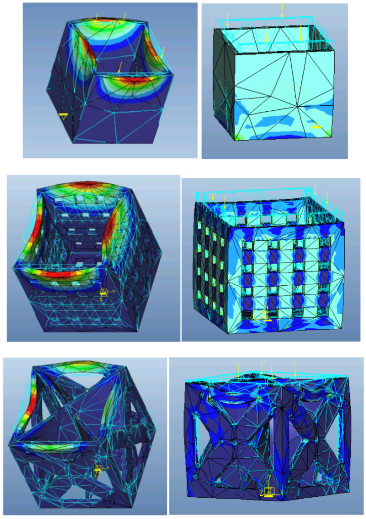
Figure 32. Geometry for the CUBE Challenge

The concrete plasticity model was adopted. Although developed to simulate primarily reinforced concrete (and in particular the micro-cracking phenomena typical in that material), this model is typically adaptable to materials exhibiting ductile behavior in compression (hardening followed by extensive softening) and brittle behavior in tension. This model assumes isotropic elasticity (with equal moduli in tension and compression) and isotropic hardening laws, but allows definition of separate tension and compression hardening laws in tabular form. The shape of the yield surface and the flo w rule can be extensively modified via a number of parameters. In the absence of calibration parameters for the material of interest, default values were chosen for most parameters. The parameters for the Concrete Damage Plasticity model were chosen as follows: Young’s Modulus, E=2.854 GPa, Poisson’s ratio, ν=0.4, Dilation Angle = 10^o, eccentricity = 0.1, fb0/fc0 = 0, K=0, Viscosity Parameter = 0. The experimental stress-strain curve for direction 3 was chosen to define the compressive hardening behavior for the entire structure, as the direction of the minimal principal stress (the compressive stress) is aligned with the z-direction for most of the structure. For the tensile behavior, the experimental curve for direction 1 was chosen for the side walls aligned with the x-direction and the two internal shells aligned with the x-direction at z=0. For the rest of the structure, the experimental curve for direction 2 was adopted. The rationale for this choice is that ABAQUS calculations revealed that the maximum principal stress (in tension) is for the most part aligned with the horizontal direction (and tangent to the local shell). The 3D CAD file was opened in SolidWorks and transformed into a shell model (Figure 32), which was subsequently imported in ABAQUS as a stand-alone part (Figure 33). Some stitching between the internal curved shells and the external walls was necessary. The bottom edges were constrained against deflection in the z-direction, as well as rotations about the x and y axes; two points were constrained against x and y translation and y translation, respectively, to kill free-body motion. The top edge was constrained against rotations about the x and y axes, and was displaced along z by 2 millimeters. All points on the top edge were constrained to deflect in z equal amounts: this (and the rotation constraints described above) simulates the presence of compression test platens. The platens will certainly exert some friction on the top and bottom edges of the cube, but good agreements with the two sample tests was obtained ignoring friction (this will result in a slightly conservative load prediction). All the structure was meshed with 8-node quadrilateral thick-shell elements, with reduced integration (S8R), see Figure 33. Nine integration points across the thickness were adopted, to improve convergence difficulties possibly related to the concrete plasticity model. The internal curved shells were assigned variable thickness along z, as prescribed by the CAD file.

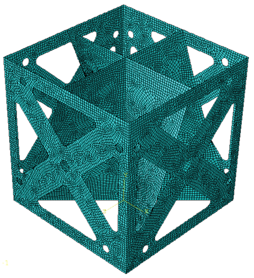Figure 33. Mesh used for the ABAQUS simulation with shell-elements

An imperfection sensitivity analysis was performed (by calculating the lowest buckling eigenmode, and introducing it in the mesh in various amounts for post-buckling (RIKS) analysis. The structure did not reveal particular imperfection sensitivity, and the best agreement for both test cases (the solid cube and the cube with side windows) resulted to be a perfect, non-perturbed mesh. A load-deflection curve obtained for the final challenge is shown in Figure 34, together with a contour plot of the plastic strain magnitude. The maximum load was recorded as 34.178kN, which is our answer for the challenge. After this point, substantial softening would occur, which resulted in convergence difficulties. The onset of convergence difficulties in the RIKS algorithm is often a sign that the maximum load is extremely close. Based on the above, our answer for the CUBE CHALLENGE is

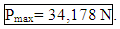
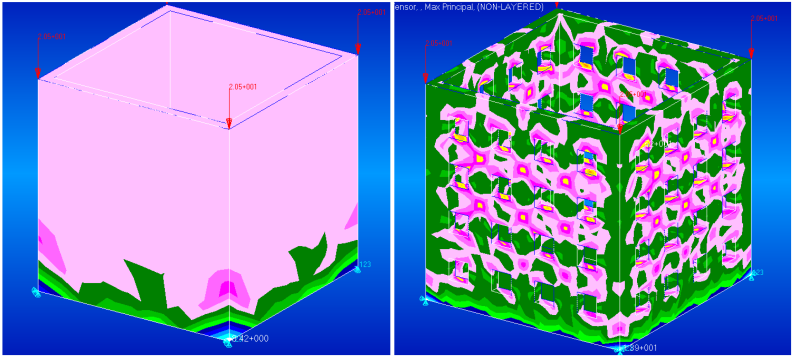
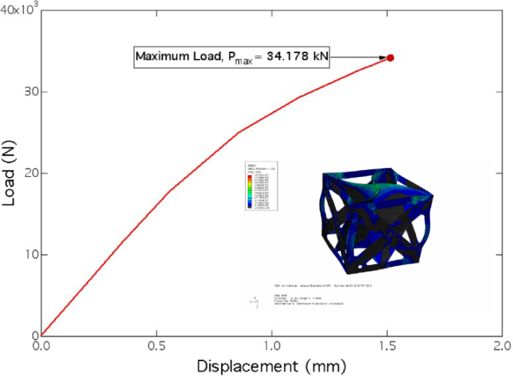Figure 34. Load-deflection curve for the cube challenge problem. The inset shows contours of the plastic strain at the maximum load

3.13.4. Titanium Sphere

Sphere prediction methodology [Scott Godfrey, sgodfrey@uci.edu].

For prediction of failure loads for the sphere models, we implemented an interactive and resume-able multi-threaded object-oriented particle swarm optimizer written in C++ with a custom swarm particle object. The goal was identifying the best polynomial fit to the posted data as a function of three variables:

with the test angle in radians, the beam velocity in mm/s, and the beam current, in mA. Four different polynomials were explored (of degrees 1 to 4), resulting in 50 fitting parameters.

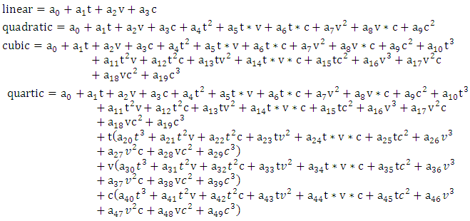On inception, the swarm objects considered every data point supplied (160+), but an identical result was obtained using just the batch-average values for each dataset (20) on the early 'practice' problems. This close correlation in predictive results indicated that the optimizer was indeed converging on useful coefficients and the extra compute-overhead of factoring all points in the clouds was unnecessary particularly in that we were predicting batch-average values. The average error was minimized over all batch data points. The average error taken as the Euclidean length of an n-dimensional vector composed of all the individual errors. Individual errors were determined as the difference in measured load relative to the corresponding predicted load. Optimizations were considered thorough and exhausted when populations in excess of 100,000 particles operating with generational life spans of 10,000 calculation cycles failed to find any predictive 'improvements' within a complete generation. Particle integration time step (value governing particle motion in normalized parameter space) was interacted with over the course of optimizations, being varied from 1.0 down to ~0.00001 as progress stagnated. Three different sets of calculations were executed, as described below.

Set1: All 20 datasets were considered with the constraint that all coefficients must be positive. Although the error was generally higher than for the other simulations, higher order polynomials (quadratic and cubic) performed best, resulting in more realistic shapes in the variables space. Additionally, all predicted loads were positive. The prediction was viable when considered relative to the nearby values.

SET1:

Coefficients were permitted to take on values in the range [0,+10e⁶]

LINEAR:

Average error: 5.07175e³ Predicted load: 2.0266e⁴ (low)

Coefficients:

QUADRATIC:

Average error: 4.89191e+003

Predicted load: 2.3030e+004 (reasonable)

Coefficients:

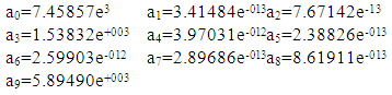CUBIC:

Average error: 4.86730e+003

Predicted load: 2.3454e+004 (reasonable)

Coefficients:

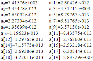QUARTIC:

Average error: 4.57712e+008

Predicted load: 1.4619e+007 (NOT REASONABLE!)

Coefficients:

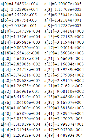Set2: Only 6 datasets were considered with the constraint that all coefficients must be positive. The solution is similar to that of set 1, but with linear and quadratic polynomials emerging.

Nearest Neighbors used (6 points):

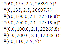LINEAR:

Average error: 4.53880e+003

Predicted load: 2.3750e+004 (reasonable)

Coefficients:

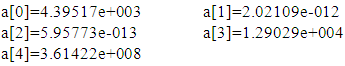QUADRATIC:

Average error: 4.53880e+003

Predicted load: 2.3750e+004 (reasonable)

Coefficients:

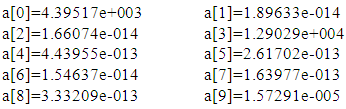CUBIC:

Average error: 1.63838e+008

Predicted load: 1.1703e+007 (NOT REASONABLE!)

Coefficients:

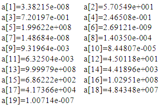QUARTIC:

Average error: 8.45203e+008

Predicted load: 1.7148e+008 (NOT REASONABLE!)

Coefficients:

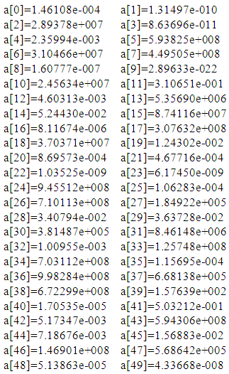Set3: All 20 datasets were considered with no constraint on the sign of the coefficients. This resulted in the smallest average error of all sets (with cubic and quartic polynomials), but also allowed for predictions of negative load values; prediction through fitting was not viable. Average errors, predicted loads, and equation coefficients for each equation are reported below:

Coefficients were permitted to take on values in the range [-10E6,+10E6]

LINEAR:

Average error: 1.82252e+003

Predicted load: 2.3997e+004 (reasonable)

Coefficients:

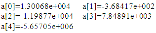QUADRATIC:

Average error: 3.05536e+002

Predicted load: 2.9967e+004 (high)

Coefficients:

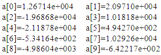CUBIC:

Average error: 5.44815e+001

Predicted load: -3.1866e+005 (BAD!)

Coefficients:

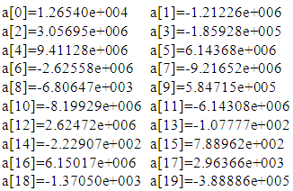QUARTIC:

Average error: 2.42912e+001

Predicted load: 5.8078e+004 (high)

Coefficients:

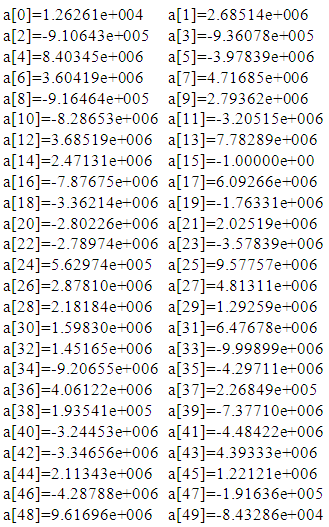Based on the above, our answer for the SPHERE CHALLENGE is

4. Summary

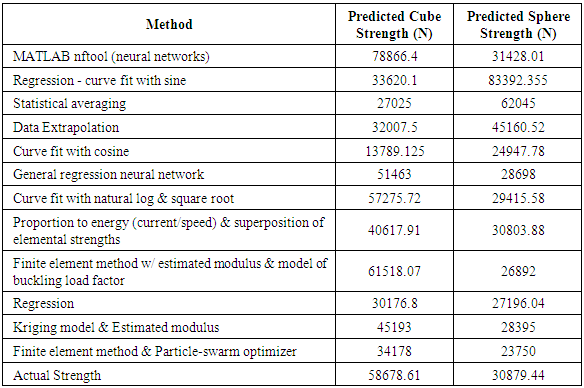
Seeking to analyze output properties of digitally manufactured components DARPA executed a Challenge on the worldwide web to any and all willing participants. Participants were challenged to develop a correlation model that accurately correlates digital manufacturing (DM) machine inputs to output structural test data. Participant models were then evaluated by their ability to predict the test results of the final DM structures. Several of the participants’ predictions are listed in Table 5 and plotted in Figure 35. The model that most accurately predicted the final test results won the Challenge. Many disparate technical approaches were investigated by researchers from all over the world, and this paper introduced readers to several of those interesting technical approaches.

Of deeper significance is the residual database of hundreds of material property tests performed on articles made with various input settings on typical DM hardware. This database remains freely available to worldwide researchers 0. Thus, the Challenge proves to merely be the simplest beginning.

Table 5. Summary comparison

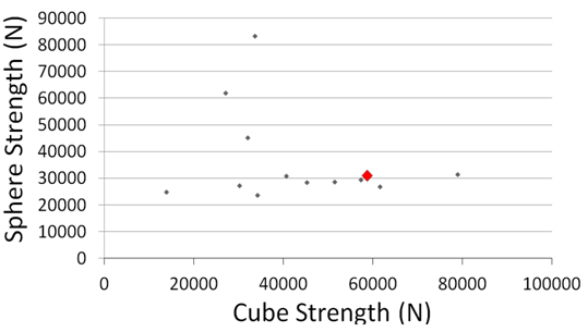Figure 35. Challenge participants’ predictions (true value in red)

ACKNOWLEDGEMENTS

The team of DARPA Fellows who conceived and executed this investigation included the author in addition to Lt Col Clinton Armani PhD, clinton.armani@us.af.mil; CDR Bill Lawerence, lefty.f14@gmail.com, Lt Col Paul Filcek, paul.filcek@us.af.mil, LTC David Rhoads, david.rhoads@us.army.mil, Joan Straub, joan.a.straub@nga.ic.gov, MAJ David Weinstein, david.weinstein@usmc.mil, and LTC Thomas Westen, twesten@cox.net. Auburn University participants include Dr. Luis Cueva-Parra, cuevadeu@yahoo.de. Data Extrapolation submission 4 participants include Robet Lenzen, e.lenzen@yahoo.com. Greystones Group participants include Jay Park Graven, jaygraven@gmail.com. Isakson Engineering participants include Dr. Steve Isakson, swi@IsaksonEngineering.com. Lamar University participants include Assistant Professor Xinyu Liu, xinyu.liu@lamar.edu. North Carolina State participants include Martin Samayoa, PhD Student, mjsamayoa@ncsu.edu. North Carolina State A&T University participants include BIEES, kj989018@ncat.edu. Pennsylvania State participants include Oyku Asikoglu，PhD Student, oxa115@psu.edu. “Snowballs Chance” submission participants include Robert Lenzen. Team Cavanaugh members include Mark Cavanaugh, mark.j.cavanaugh@gmail.com, and Dr. Steven Cavanaugh, info@iis-corp.com. Team PAM consists of the following members: John Porter (team leader) – jrporter@uci.edu; Lorenzo Valdevit (cube lead) – Valdevit@uci.edu; Scott Godfrey (sphere lead) - sgodfrey@uci.edu; Randall Schubert - randallcs@gmail.com; Eric Clough - eclough@uci.edu; Ed Tackett - etackett@rapidtech.org; Ken Patton - kpatton@rapidtech.org John Wooten - john.wooten@calraminc.com. University of California, Santa Barbara participants include Frank Zok, zok@engineering.ucsb.edu, PhD students Nell Gamble and Chris Hammetter, as well as Professor Matt Begley. University of Missouri-Columbia participants include Brian Graybill, PhD Student, bsgmr2@mail.missouri.edu. Washington University in St. Louis participants included Marcus Richards and the “Eccentric Crushers” from the Student Section of the American Society of Mechanical Engineers, marcus.richard.l@gmail.com.