1. Introduction

1.1. Background

The purpose of this research includes using a National Instruments [1, 9] myDAQ [2] to read and process signals from a piezoelectric film element [3, 10]. See Figure 1. The goal of the paper is to stand as an easy-to-follow guide to experimental system identification with many illustrations to help investigators duplicate the procedure and results. A piezoelectric element is configured as a cantilever [4], which is bent by a motor and cam assembly [5]. Due to the piezoelectric effect, the strain created by the mechanical displacement [6] generates charges in the piezoelectric material, which are translated to a voltage reading with a charge amplifier circuit [7]. This article takes the reader through a rigorously documented procedure to duplicate experiments that distinguish real data from other factors that often confound theorist seeking to apply their knowledge experimentally: 1) additional response data induced by signal measurement, 2) signal harmonics, and 3) signals induced by the power supply. We’ll start by investigating the effect of Rref, Cref (reference resistance and capacitance respectively) and the time constant of the intended circuit [8].

1.2. Literature Review

Space radar structures [11] utilize smart structural control of lightweight spacecraft using piezoelectric elements begin with controlling the rigid body dynamics (equation (1) in [13]) that are disturbed by rotating attitude control actuators [12, 13, 15, 17, 20, 25, 27]. Especially to avoid control-structural interaction, flexible appendages and robotic manipulators are included by adding the flexible dynamics to the rigid body dynamics. In order to account for imprecise estimates of the dynamic properties, nonlinear adaptive controllers are a logical next step [13, 16, 19, 21-24, 26, 28-32] that include online system identification algorithms [30-32]. These algorithms perform ubiquitously better when initialized by good estimates of system parameters, making a priori system identification very important. Taken together, these methods provide effective control of lightweight, flexible space structures with fine pointing supporting wide-array radar employment [11, 14, 18] or optical imaging.

1.3. Formulation of the Problem of Interest for This Investigation

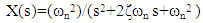
This research focuses on the a priori estimation of natural frequencies of the piezoelectric elements of robotic appendages of spacecraft. The rigid body dynamics expressed in equations (1)-(6) in reference [13]. The rotating actuator disturbance dynamics are expressed equations (7)-(11) of reference [13] and equations (1)-(3) in reference [20]. The nonlinear adaptive control equations are displayed in equations 1-6 of reference [32]. These online system identification algorithms require good estimates of system parameters, one of which is the natural frequency of the piezo electric element which embodies the mass and stiffness properties of the element per equation (1) below:

(1)

The stiffness is a relationship between the applied force and resultant displacement per equation 2, in this case bending displacement of the cantilever piezo element.

(2)

Thus, the most important measure is accurate displacement. Later in the Methods section, the piezo displacement relationship will be revealed as a second order mathematical equation that will be used to solve for the natural frequency given experimental deflection data.

1.4. Contribution in this Study

The contribution to this study lie in illustration of real-world techniques to implement measures necessary to maximize performance of online, nonlinear-adaptive control of highly flexible spacecraft using piezoelectric elements and sensors and potentially actuators for controlling ultra-lightweight, highly flexible spacecraft appendages. The uniqueness lies in the actual laboratory system identification procedures to initialize the dynamic, nonlinear adaptive controllers that are based on the mathematical system models.

1.5. Organization of this Paper

Following this introduction, the paper will immediately describe very detailed procedures to perform real-world system identification using in expensive laboratory hardware. Very detailed procedures are articulated to maximize repeatability, and results are given for various logical configurations, even when the results are poor, highlighting relatively good and bad configurations for experimental analysis in both time domain and frequency domain, where particular attention is given to power supply voltage while spectral contributions from power supply are highlighted to prevent the reader some erroneously inferring the identified frequency content in the experimental signal. The result will illustrate that increased supply voltage produces superior data plots. Next, using operational amplifiers as circuit buffers is investigated as another option for superior plots of spectral content with iterations for various reference capacitance and reference resistance values. In addition to providing experimental results for each iteration in data plots, the results are summarized in data tables to allow numerical comparison including two commonly available operation amplifiers.

2. Materials, Methods, and Results

A motor and a plastic cam mounted on the motor are used to cyclically bend a piezoelectric cantilever. See Figure 1 & Figure 2. The piezoelectric cantilever is deflected slightly, once per revolution generating a voltage. The piezoelectric element has two electrode contacts and has been mounted on one side of a DIP (dual in-line pin) IC socket.

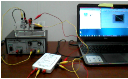Figure 1. myDAQ connected to piezo element

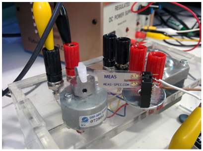Figure 2. Hardware configuration

2.1. Estimate Motor Rotational Rate

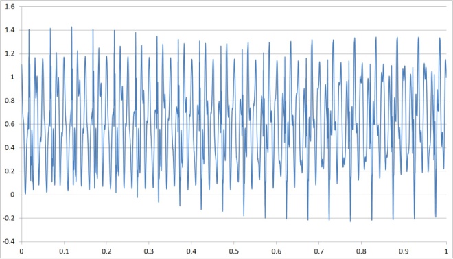
We can estimate the rotational rate of the motor by simply noting the time it takes the motor to accomplish one revolution (the time between spikes in voltage measurements) as displayed in Figure 3 where the motor is being fed 1.5V, 1A source. Set the probe to 1X (corresponding to an input resistance of 1 MΩ). You also need to adjust the oscilloscope to reflect this setting: Press Ch1 Menu and change the Probe setting to 1X. For easier reading, you can press the Run/Stop button to freeze the waveform.

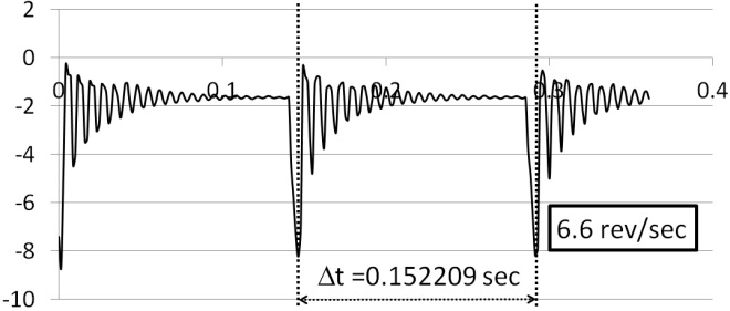Figure 3. Estimating motor speed: time vs. deflection amplitude

The myDAQ was used as an oscilloscope [9] at the probe was set to 1X corresponding to an input resistance of 1MΩ. The program used to collect data is depicted in Figure 4. The ambient response was plotted (Figure 5) prior to activation of the motor to understand the portion of the response that was provided by the myDAQ. When the motor is provided 1.5V and the oscilloscope is set to 1MΩ the results are depicted in Figure 6.

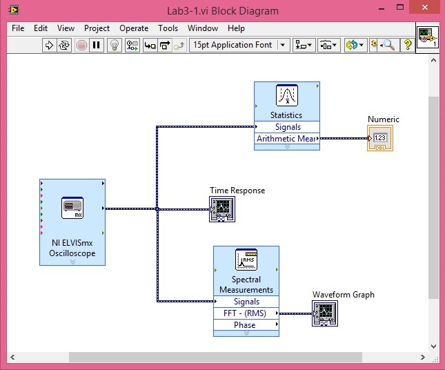Figure 4. Software configuration

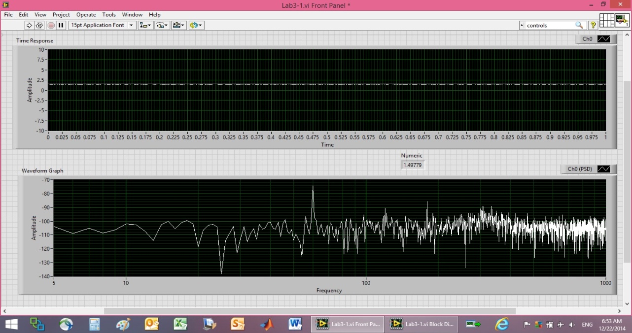
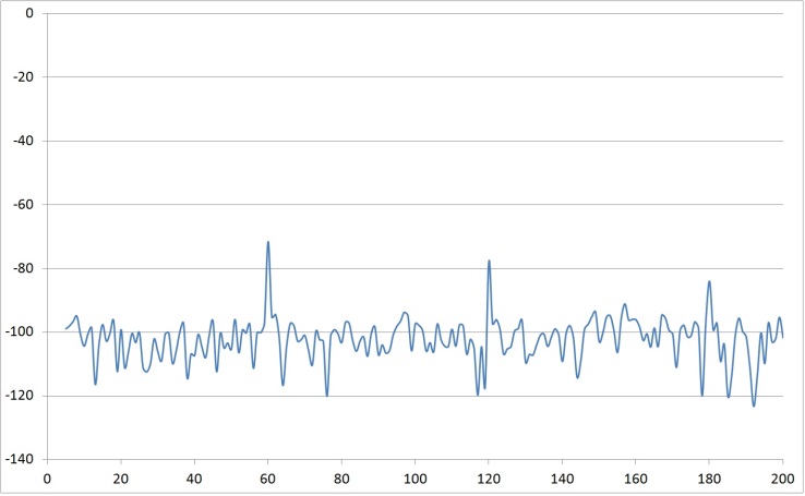
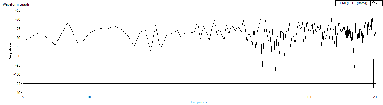
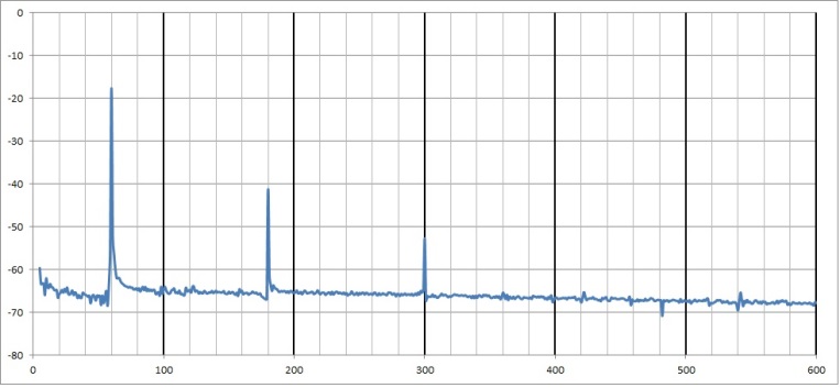Figure 5. Ambient response due to myDAQ: frequency vs. response amplitude

Figure 6. Oscilloscope at 1MΩ, motor at 1.5V: time vs. deflection amplitude

The piezo element is a second order system [10] per Equation 3. The mechanical deflection of the piezo with periodic impulses may be modeled by a mass-spring-damper system or alternatively by a RC circuit. Assuming the under-damped case, 0<ζ<1, and the time-response behaves per Equation 4 where the natural frequency ωn may be estimated using the impulse response by measuring the time between subsequent peaks. See Figures 7&8 which reveals an estimate of natural frequency.

(3)

(4)

Notice the peak around ω_n=898Hz (pretty close to the second estimate) is joined by two other peaks indicating there are other frequencies present in the voltage signal. Speaking coarsely, consider the natural frequency is around 900…half of 900 is 450…and we see a peak of energy around 450Hz. One-third of 900 is 600, and we see a peak around 600Hz. Thus, the two other spikes are likely fractional-ordered harmonics of the natural frequency. This will be discussed further in all the subsequent sections.

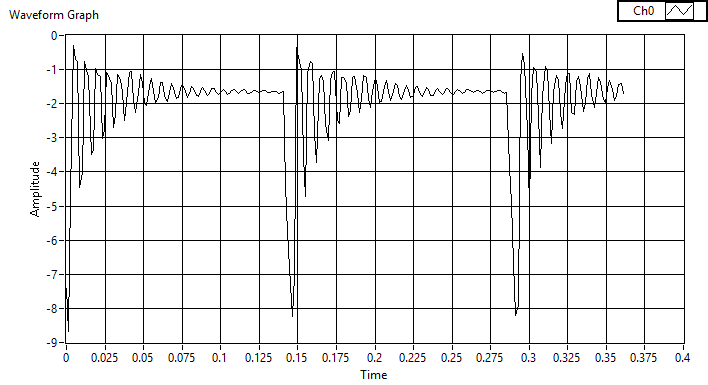
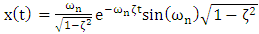
Figure 7. Estimating ωn by time-between peaks: time vs. deflection amplitude

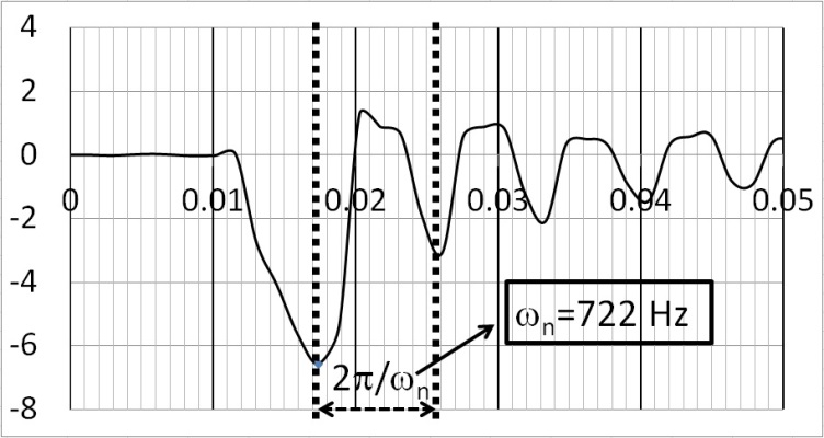
Figure 8. 2nd Estimate of ωn: time vs. deflection amplitude

Figure 9. FFT reveals ωn & other spectral content: frequency vs. response amplitude

2.1.1. Set Probe to 10X

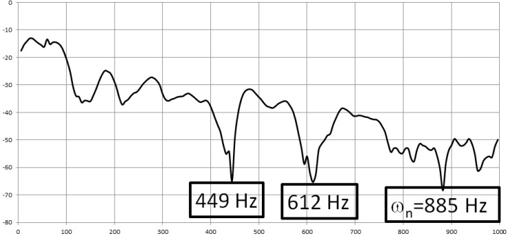
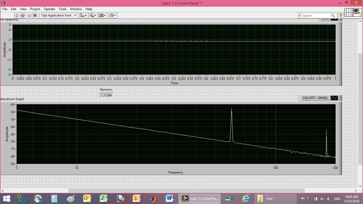
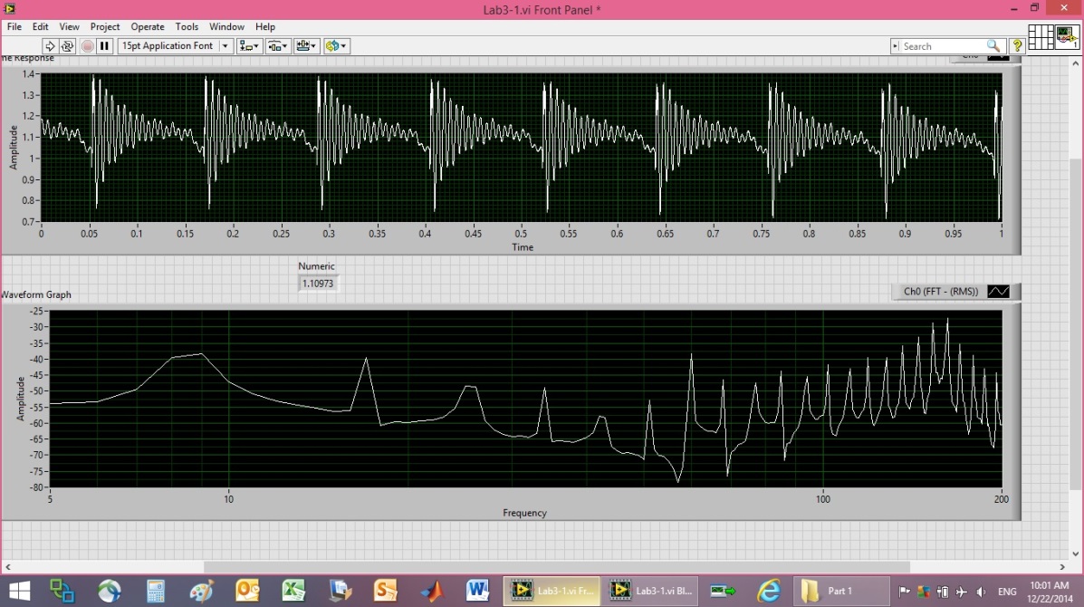
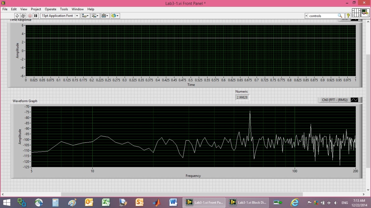
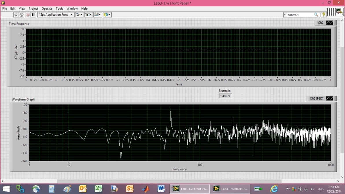
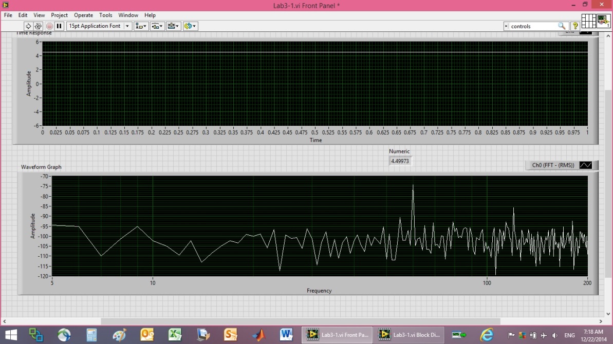
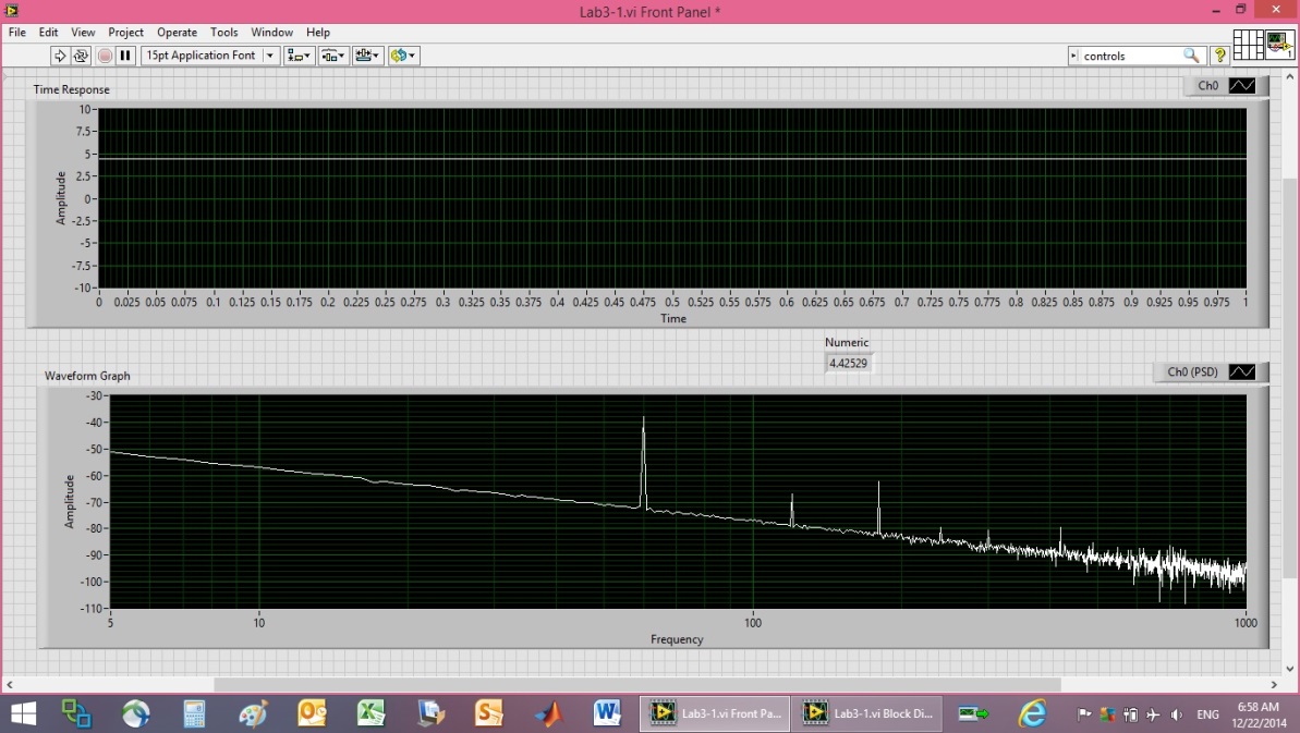
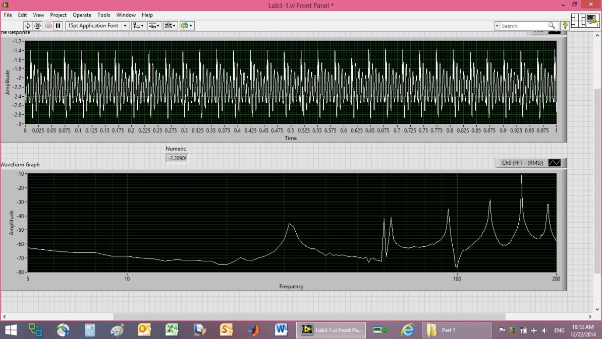
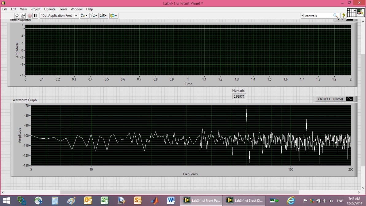
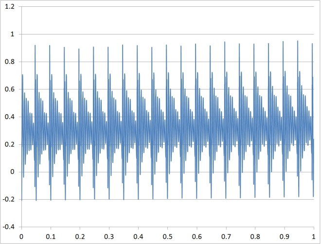
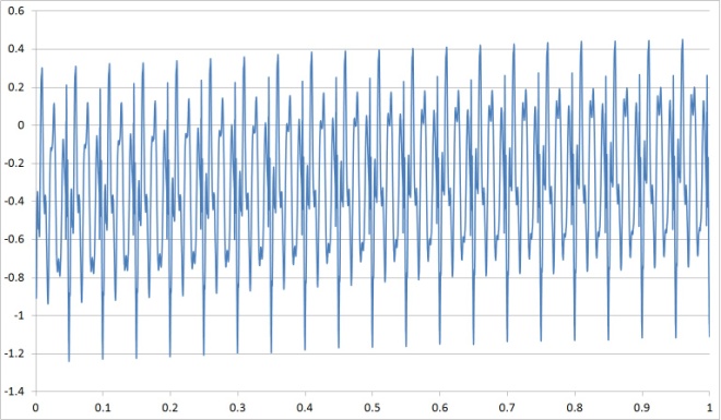
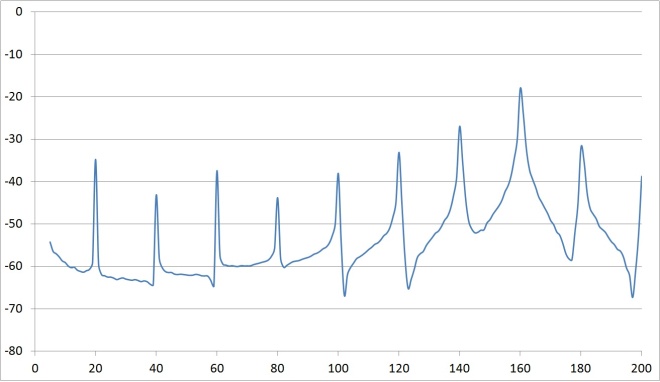
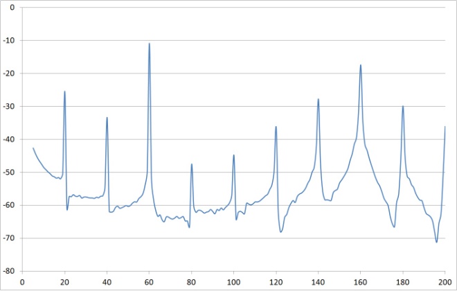
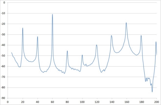
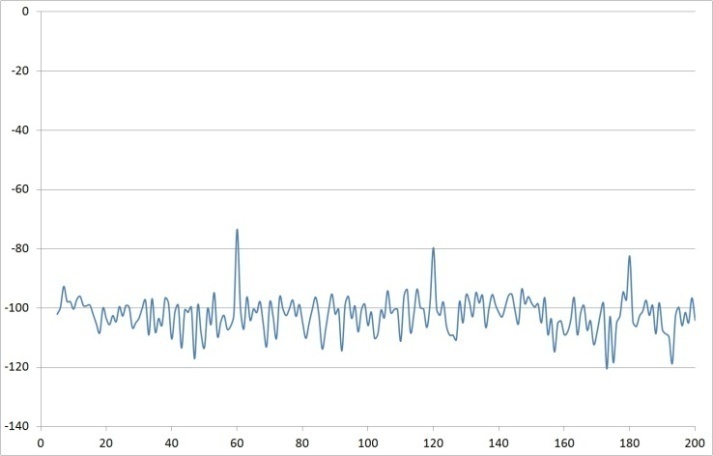
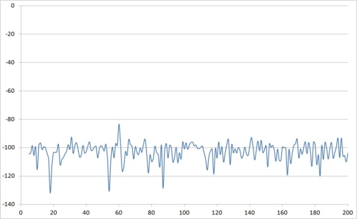
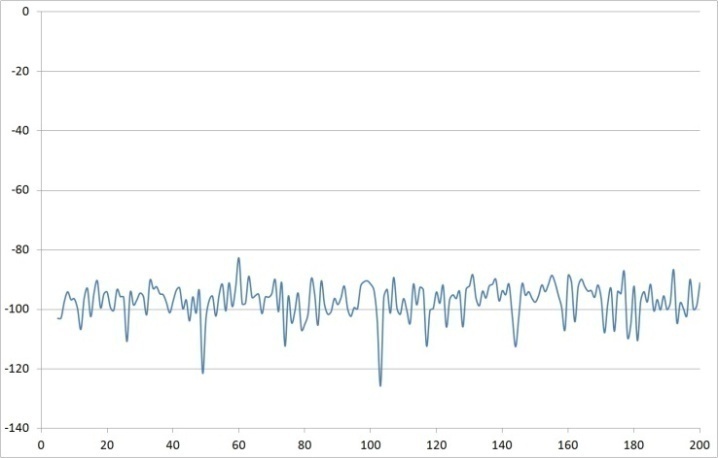
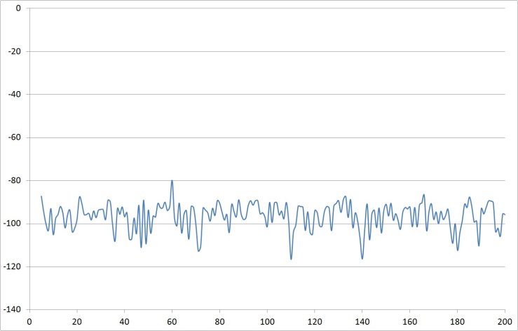
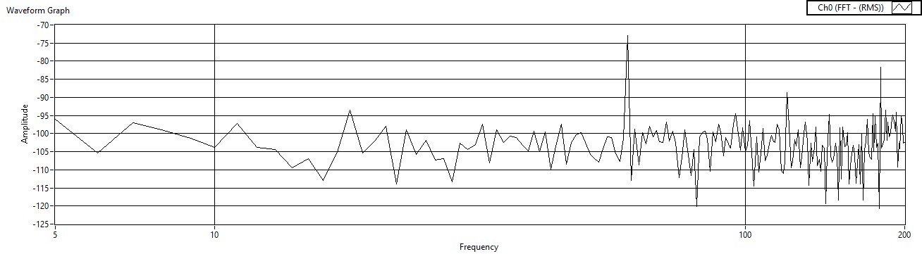
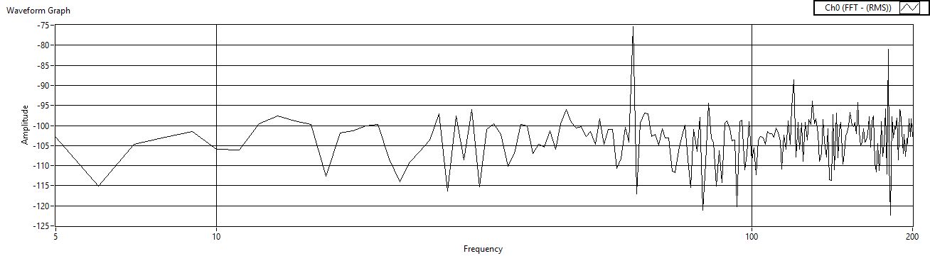
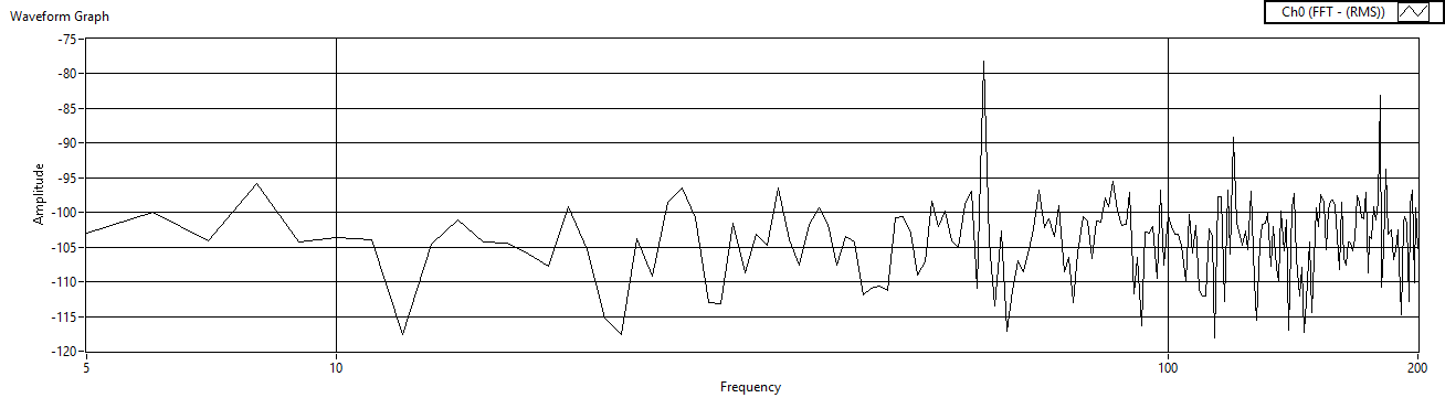
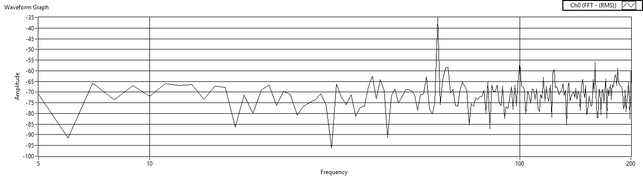
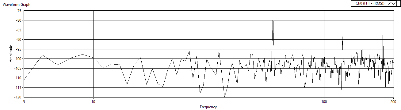
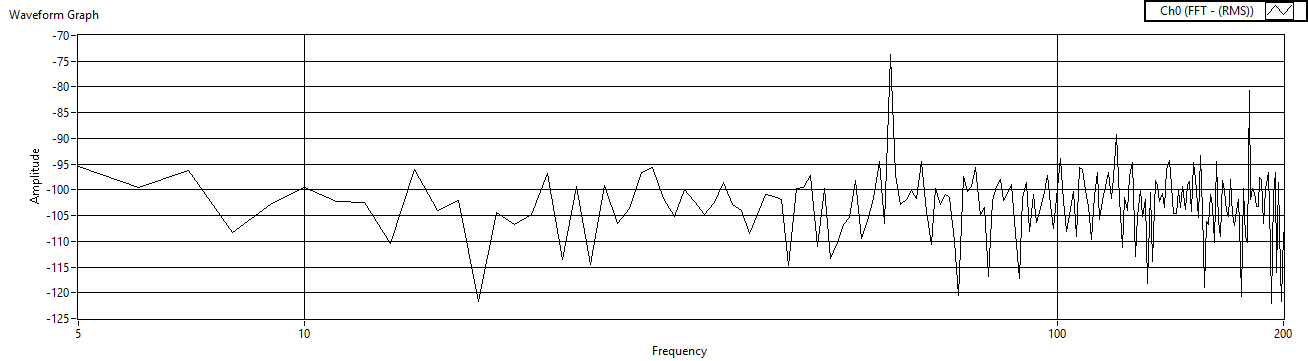
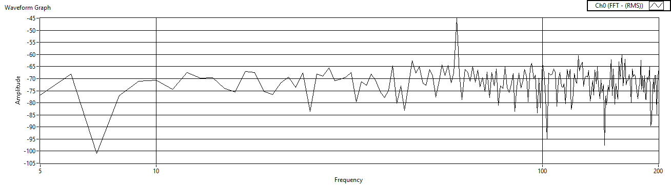
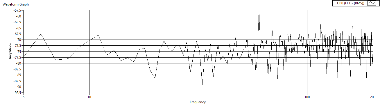
Zoom the depiction around 200Hz. Do you experience saturation above 5V? Regardless, the following plots depict a repositioned piezo element with varying applied voltages (1.5V, 3V, 4.5V, and 6V). The frequency response data is pretty bad at first, but with increasing voltage the plots improved (ref: Figure 10 - Figure 17, Figure 19). Setting the probe to 10X changes the oscilloscope input resistance to 10MΩ. Continue to compare 1X, 10X, and using myDAQ for >10GΩ.

As described earlier, the frequency response data is very poor at 1.5V, and the resonances are not easily discernible. On the other hand, at 6V it is easy to see resonances just over 40Hz, exactly at 60 Hz (clearly due to the power supply), just over 80 Hz (likely harmonically linked with the signal at 40Hz), a resonance just over 100Hz (120Hz seems more theoretically likely if its linked to the 60 Hz signal), and another up near 160 (again probably harmonically linked to the signals at 40 and 80Hz). Since the 160Hz peak is largest: Based on Figure 19, ω_n~160Hz.

Figure 10. 1.5V Power supply calibration plot

Figure 11. myDAQ calibration at 1.5V

Figure 12. 1.5V Piezo Output data

Figure 13. 3V Output calibration plot

Figure 14. 3V Piezo Output data

Figure 15. 4.5V Power supply calibration plot

Figure 16. 4.5V myDAQ calibration at 1.5V

Figure 17. 4.5V Piezo Output data

Figure 18. 6V Power supply calibration plot

Figure 19. 1.5V Power supply calibration plot

2.2. Add LMC6484 op-amp as Buffer Circuit

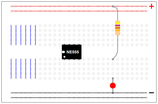
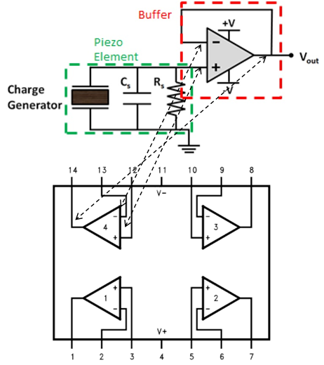
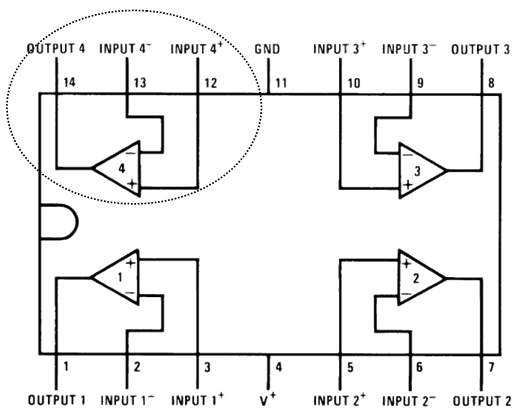
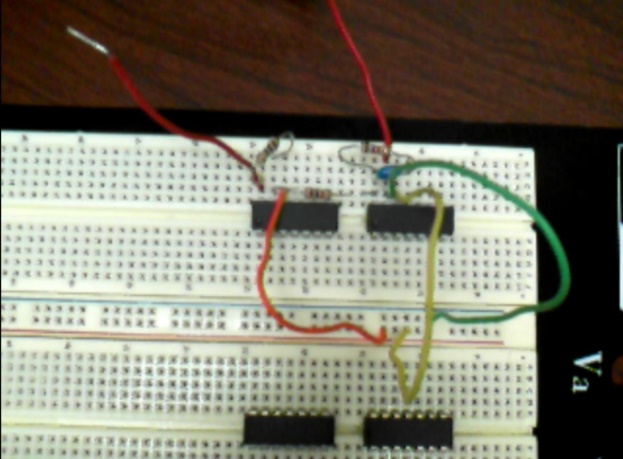
In the first part of this article, we saw that we could increase the supply voltage to clean up the frequency response data. Another option is to include amplification in the circuit as opposed to increasing the supply voltage. The next part of the laboratory research utilized an LMC6484 operational amplifier (op-amp) in Figure 22 as a buffer circuit. Op-amps are particular useful to filter signals as well as add or subtract offsets and apply gain amplification. Notice in Figure 20 how we construct the circuit on a breadboard.

Figure 20 is an illustrative example of a breadboard. The blue straight lines on the left side of the breadboard indicate holes in the surface that are all connected. The upper and lower lines that run left-right also indicated connected holes. Connections are emphasized, since that’s how breadboards are built.

Figure 20. Example of breadboard connections

First, examine the circuit diagram that we wish to construct on the breadboard, paying particular attention to the connections. Then, implement these connections on the breadboard where you reserve the outer left-right running holes to establish voltage supply and ground (+/-) signals. Figure 21 depicts an op-amp in a “buffer” configuration, where the positive end of the op-amp is connected to the positive end of the piezo element. Connections are then mimicked from Figure 21 onto Figure 20. Figure 22 reveals the pin-connections for the LMC6484 op-amp. In the experiments discussed in this article, pins 12-14 were used.

Figure 21. “Buffer” configuration of op-amp & Figure 22. Figure 22. LMC6484 Pin diagram

Referencing Figure 21, notice the op-amp inputs are the same, and connected to V_out. Thus, we can connect almost anything that draws current to V_out of the buffer and it won’t interfere with the current in the piezo element to the left, i.e. they are isolated (thus the name “buffer”). The non-inverting input draws no current, and so the output is driven by the op-amp. If you connect anything that draws current to the piezo element on the left, you’ll distort the current (called “loading”), essentially changing the voltage by measuring it. So, here we’ve instead used an op-amp “buffer” to connect current-drawing devices to the right without drawing from the high impedance source on the left.

Especially since op-amps draw no current, the output in this negative feedback configuration does whatever is necessary to make the voltages at the inputs be equivalent. Thus we anticipate some interesting signals measured at the op-amp output (aka “read” by the buffer) as compared to measuring the output at oscilloscope (at the op-amp input). The 5V fixed supply was connected to the op-amp, and the variable power supply was used to power the motor at 3V. The piezo was put into a position to insure saturation avoidance at 5V. Afterwards, the piezo was screwed into place very tightly in order to normalize the experiments for the remained of the investigation.

Measurements were taken from the oscilloscope and also from the buffer, and the two were compared (depicted in Figure 23 and Figure 24). As described, the buffer output is doing whatever is necessary to the signal to make the voltages at the inputs be equal. It is certainly apparent in the figures, using a buffer did not improve the appearance of the time-response. Next, consider the frequency response. Figure 25 and Figure 26 display the frequency response data that accompanies the time-response data displayed earlier in Figure 23 and Figure 24 respectively. Notice the resonant peaks are amplified. So, cone benefit of using the op-amp as a buffer was enhanced frequency response measurement with nominal input voltage.

Figure 23. Time vs. response read by oscilloscope

Figure 24. Time vs. response read by buffer

Figure 25. Time vs. response read by buffer

Figure 26. Time vs. response read by buffer

2.2.1. Add LM324 op-amp as Buffer Circuit

Next, the same procedures was performed as part a, but this time the LMC6484 was replaced with a LM324 op-amp displayed in Figure 27. The pin-configuration is quite similar, and again the upper-left pins (12-14) were used. The time-response plots were similar using either op-amp, but the frequency response plot was superior using the LMC6484 op-amp. The LMC6484 response was slightly better than the LM324 response.

Figure 27. LM324 Pin diagram

Figure 28. Time vs. Buffer-read Time-Response

Figure 29. Frequency vs. Buffer-read Frequency Response

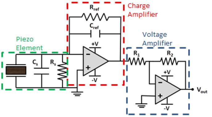
2.3. Experiments with a Charge Amplifier

Next, add a charge amplifier by adding an inverting amplifier after the buffer (charge amplifier), where voltage is amplified by a gain established by the ratio of resistors per equation 5.

(5)

A gain value of R₂/R₁=1000 is established by R₂/R₁=1MΩ⁄1kΩ. Place these resistors on the breadboard per Figure 30 and Figure 31.

Figure 30. Circuit schematic corresponding to figure 31

Figure 31. Circuit implementation corresponding to figure 30

The two red wires in Figure 31 indicate where measurements are taken (“at the oscilloscope” versus “at the amplifier”). The center two left-to-right rows of holes in the breadboard in Figure 31 are connected to the 3V fixed power supply (see Figure 32). The upper two op-amps active in the depicted circuit in Figure 31 are LMC6484 op-amps, while the lower to are LM324 op-amps. Next, in section 2.4, we’ll investigate the LM324, so the circuit was simply built around the lower portion of the breadboard as it was earlier in the depicted circuit in the breadboard.

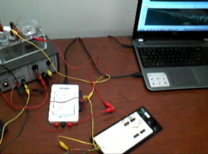Figure 32. Lab hardware setup with charge amplifier

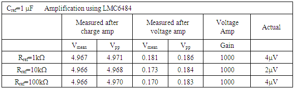
2.4. Investigate Reference Resistance

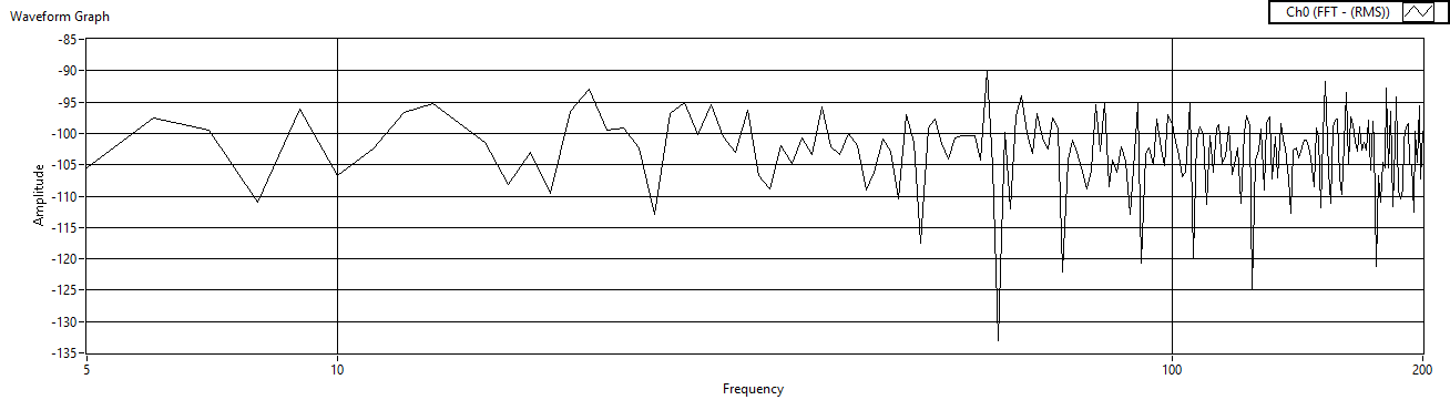
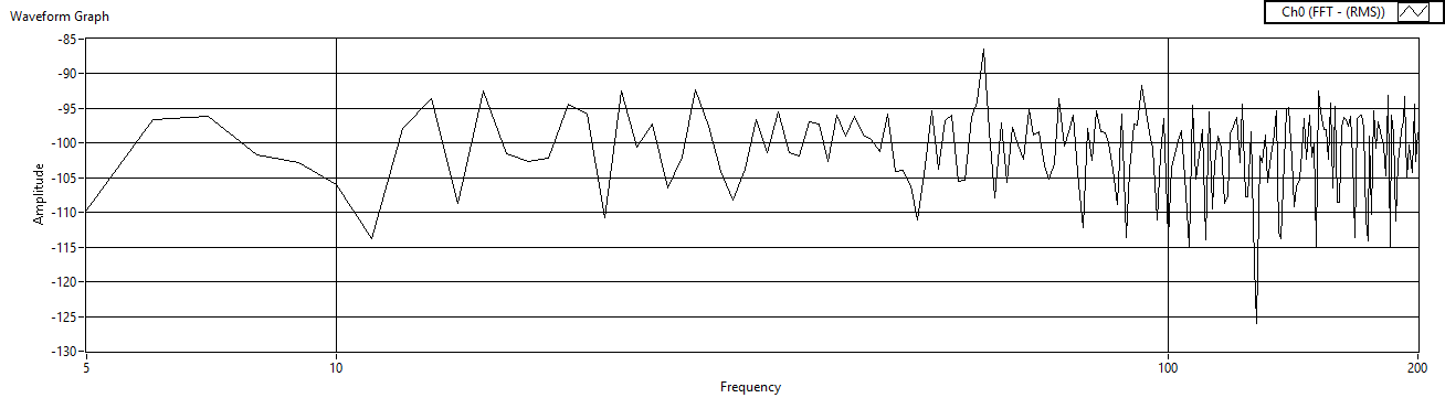
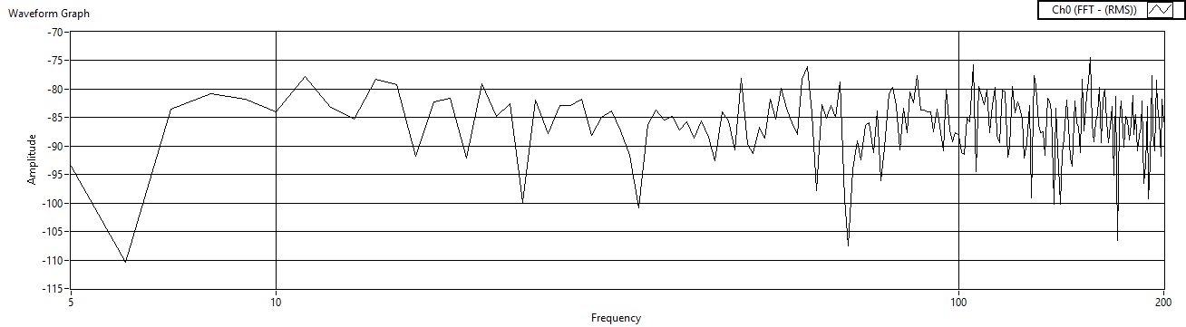
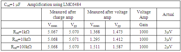
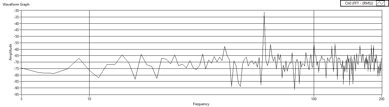
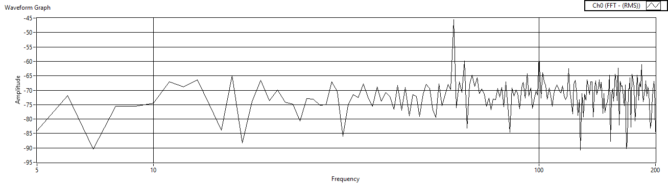
Next, investigate reference resistance by fixing the reference capacitor and the gain resistors, and then iterate the reference resistor. The experimental results are listed in Table 1 and figures 33-38.

Table 1. Iterated reference resistor results

The measurements before voltage amplification were essentially identical for all three reference resistors; however the measured voltage after voltage amplification gradually decreased with increasing reference resistance. As we saw earlier, the addition of the op-amps degraded our measurement of the time-response, but improved our frequency-response measurement without increasing supply voltage. Frequency response plots are provided in Figure 33 - Figure 38 to investigate potential improvements with iterated reference resistance. The three iterated cases after charge amplification are presented in Figure 33 - Figure 35 to reveal that the three resonant peaks have improved display (reduction of spike-levels elsewhere). On the other hand, measurement after voltage amplification does not provide benefit (see Figure 36 - Figure 38). All spikes were reduced with increasing reference resistance.

Figure 33. Rref=1 time vs. response measured after charge amp

Figure 34. Rref=10 time vs. response measured after charge amp

Figure 35. Rref=100 time vs. response measured after charge amp

Figure 36. Rref=1 time vs. response measured after voltage amp

Figure 37. Rref=10 time vs. response measured after voltage amp

Figure 38. Rref=100 time vs. response measured after voltage amp

2.4.1. General Conclusion

Use buffer-alone for clean voltage plots, use buffer with voltage amplifier to clean up frequency plots, taking measurements before voltage amplification.

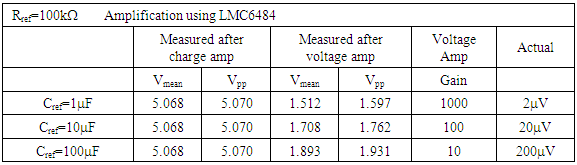
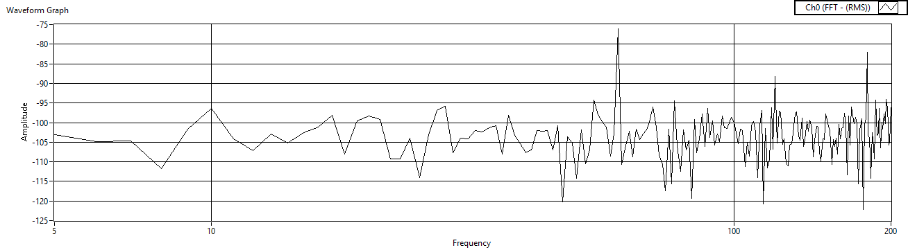
2.5. Investigate Reference Capacitance

Next, fix the reference resistor and the gain resistors, and then iterate the reference capacitor. The experimental results are listed in Table 2.

Table 2. Iterated reference capacitor results

One real benefit is tripling of the voltage signal (minus offset) when using a voltage amplifier. The measurements before voltage amplification were again essentially identical for all three reference resistors; however this time the measured voltage after voltage amplification also remained unchanged with increasing reference resistance. Thus, the resistor, not the capacitor has a relatively larger effect on the measured voltages.

As we saw earlier, the addition of the op-amps degraded our measurement of the time-response, but improved our frequency-response measurement without increasing supply voltage. So, again I’ve opted to provide frequency response plots are provided in Figure 33 - Figure 38 to investigate potential improvements with iterated reference resistance.

On the other hand, measurement after voltage amplification does not provide much benefit (see Figure 39 - Figure 44) with respect to frequency response display. All spikes were not reduced with increasing reference capacitance as we saw with reference resistance.

Figure 39. Cref=1μF measured before charge amp

Figure 40. Cref=10μF measured before charge amp

Figure 41. Cref=100μF measured before charge amp

Figure 42. Cref=1μF measured before voltage amp

Figure 43. Cref=10μF measured before voltage amp

Figure 44. Cref=100μF measured before voltage amp

2.6. Iterate R_ref (w/LM324)

Next, fix the reference capacitor and the gain resistors, and then iterate the reference resistor, but this time replacing the op-amp with a LM324 op-amp. The experimental results are listed in Table 3 with iterations displayed in Figure 45 – Figure 50.

Table 3. Iterated reference resistor results

Figure 45. Rref=1 measured after charge amp

Figure 46. Rref=10 measured after charge amp

Figure 47. Rref=100 measured after charge amp

Figure 48. Rref=1 measured after voltage amp

Figure 49. Rref=10 measured after voltage amp

Figure 50. Rref=100 measured after voltage amp

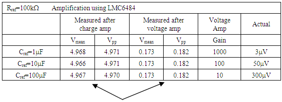
2.7. Iterate C_ref (w/LM324)

Finally, fix the reference resistor and the gain resistors, and then iterate the reference capacitor. The experimental results are listed in Table 4 and the results are displayed in Figures 51 – Figure 56.

Table 4. Iterated reference resistor results

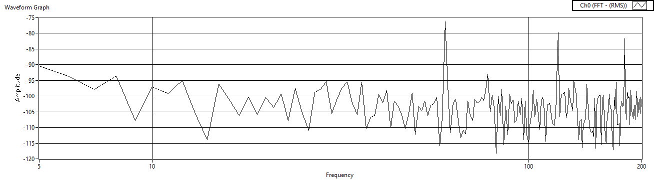
Figure 51. Cref=1μF measured after charge amp

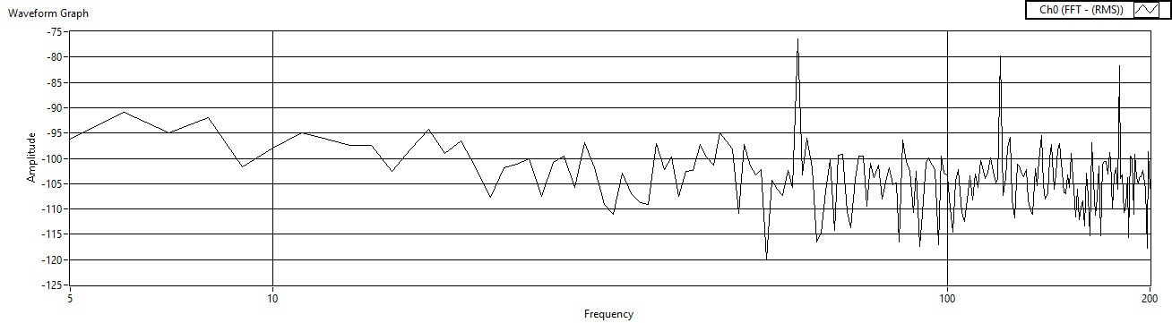
Figure 52. Cref=10μF measured after charge amp

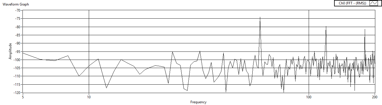
Figure 53. Cref=100μF measured after charge amp

Figure 54. Cref=1μF measured after voltage amp

Figure 55. Cref=10μF measured after voltage amp

Figure 56. Cref=100μF measured after voltage amp

3. Results and Discussion

The oscilloscope does a really good job of displaying the time response (see Figure 6), but the spectral data was more suspect (noting several different natural frequencies dependent upon the hardware setup). Especially since system ID largely comprises identification of the natural frequency, it is preferred to not modify the measured signal (as is the case with the oscilloscope). Furthermore, improved spectral plots result with increased supply voltage (re-examine Figure 19’s spectral plot!) which is not always a good thing. Therefore we next investigated using buffers. The buffer provided improved spectral data, but the buffer output did whatever was necessary to the signal to make the voltages at the inputs equal (again placing us on the path of modifying the signal). Note the difference between Figure 23 and Figure 24. Using the op-amps in the buffer configuration resulted in pretty spectral plots, but there were lots of “ghost” resonances. Using the op-amps in the two-stage charge amplifier configuration suppressed the “ghost resonances”. In all cases, taking measurements at the output of the charge amplifier was superior to taking measurements at the voltage amplifier. The two-stage amplification configuration provided on the order of triple voltage signal (peak minus offset) amplification. Several of the iterated cases provided good signal amplification with very legible spectral data plots. The LMC6484 response was slightly better than the LM324 response in the buffer configuration, but the opposite was true in the case of the two-stage amplifier configuration.

This experimental analysis reveals practical techniques for experimental system identification, in particular of natural frequencies of piezoelectric elements that are useful to control very light, highly flexible space appendages that complicate attitude control, especially instances where controls-structural integration occur.

4. Summary and Conclusions

Utilizing the methods in this paper, the reader can accurately estimate system parameters of piezoelectric elements that can be used to aid the control of highly flexible space structure. The system estimates can be used to initialize nonlinear, adaptive attitude control methods based on the system mathematical models that control both the rigid body modes and flexible modes of the spacecraft dynamics. Well-initialized adaptive controllers are able to achieve high pointing accuracy facilitating operational missions such as space radar and optical payload support.

ACKNOWLEDGEMENTS

This investigation was guided by Stanford’s Tom Kenny’s calling to provide working knowledge of modern actuator technologies. Furthermore, all experimental results were achieved using Professor Kenny’s laboratory equipment.