Naoto Kobayashi, Mai Bando, Shinji Hokamoto
Department Aeronautics and Astronautics, Kyushu University, Fukuoka, Japan
Correspondence to: Naoto Kobayashi, Department Aeronautics and Astronautics, Kyushu University, Fukuoka, Japan.
| Email: |  |
Copyright © 2017 Scientific & Academic Publishing. All Rights Reserved.
This work is licensed under the Creative Commons Attribution International License (CC BY).
http://creativecommons.org/licenses/by/4.0/

Abstract
This study discusses motion estimation processes for vehicles by Wide-Field-Integration (WFI) of optic flow. Optic flow is a vector field of relative motion between the vehicle and environment, and WFI of optic flow is a bioinspired estimation method to make it robust even for unknown environments. This paper re-examines the form of sensitivity functions used in the WFI of optic flow, which plays a key role in the robust estimation process. Furthermore, since optic flow is obtained from real image sensors, the effects of several restrictions of practical sensors are investigated in numerical simulations. Finally, the effectiveness of the proposed form of sensitivity functions is experimentally verified by using real sensors boarded on a flying vehicle.
Keywords:
Motion Estimation, Optic Flow, Wide Field Integration, Sensitivity Functions, Autonomous Navigation
Cite this paper: Naoto Kobayashi, Mai Bando, Shinji Hokamoto, Improvement of Wide-Field-Integration of Optic Flow Considering Practical Sensor Restrictions, Journal of Mechanical Engineering and Automation, Vol. 7 No. 2, 2017, pp. 53-62. doi: 10.5923/j.jmea.20170702.04.
1. Introduction
Recently the requirements of autonomous navigation systems for flying vehicles are significantly increasing. One typical application of such systems is Micro Air Vehicles (MAVs). MAVs are being actively researched in various applications to agriculture, industry, military affairs and so on. However, most of autonomous flight systems of MAVs rely on the signals of Global Positioning System (GPS). Thus, in GPS-unavailable environments such as inside of buildings, other guidance and navigation system is required for autonomous flight. One possibility for autonomous navigation is a laser sensor, but the information obtained is only the distance of an object being along to the laser beam. Furthermore, the weight and energy consumption of the sensor easily become difficulties for MAVs. Although an ultrasonic sensor is another possibility, the measurable range of the distance to environments is restricted.Wide-Field-Integration (WFI) of optic flow is considered as a promising navigation technique for autonomous flight of MAVs. That is a motion estimation method inspired by a biological research on the visual processing systems of flying insects’ compound eyes. Optic flow is the vector field of relative velocities to environments, and which is obtained by photoreceptors on image sensors boarded on a vehicle [1, 2]. In the WFI of optic flow, integration over a wide region of optic flow makes the motion estimation robust to even unknown environments. This method has several preferable features for navigation of MAVs: the system can be composed of a small-sized, light-weighted image sensor and an onboard microprocessor because of low computational requests [3-7]. In the WFI of optic flow, “sensitivity functions” in the space integration over a wide region of optic flow play a key role in the estimation process. However, the physical meaning of the sensitivity functions is not definite. Furthermore, the estimation theory for WFI of optic flow assumes that a whole directional optic flow on a spherical image surface can be obtained, and all of the obtained optic flow is integrated to estimate the vehicle’s motion parameters [8-11]. Since such integration process in real time is not realistic for an onboard microprocessor, the author’s group has proposed to replace the integration by a Riemann sum and shown that the estimation accuracy of the non-integrated procedure is not deteriorated [12]. This paper, first, re-examined the form of sensitivity functions used in the WFI of optic flow, considering the relation of optic flow components and the sensitivity function. Then, since optic flow is obtained through computer vision processing for standard camera image sequences, the practical restrictions of image sensors affect the estimation accuracy of the WFI of optic flow. Thus, the effects of integration region, the number, and the distribution pattern of optic flow are investigated in numerical simulations. Finally, the effectiveness of the proposed form of sensitivity functions is experimentally verified by using real sensors boarded on a flying vehicle.
2. Estimation from WFI of Optic Flow
2.1. Optic Flow
To describe the motion of a vehicle flying over a terrain, let define two reference frames; an inertial frame Ft fixed to the terrain and the vehicle fixed frame Fb whose origin is placed at the center of gravity of a vehicle (Figure 1). The optic flow is the vector field of relative velocities between the two frames and obtained by photoreceptors in an image sensor. Let assume that the image surface is a sphere around the center of gravity of a vehicle, and the spherical imaging surface is denoted with  The position of photoreceptors on the spherical surface is described with two angles: the azimuth angle
  and the elevation angle
  which are measured positive from the xb- and zb-axes of the frame Fb, respectively. Then the line-of-sight vector for each photoreceptor is denoted as follows:
 | (1) |
The fiducial point on the terrain is assumed stationary to the reference frame. Then, the motion parallax vector  is defined as the time derivative of
  on the spherical imaging surface, which is generated according to the vehicle’s translational and rotational motion. Let v = [u v w]T be the translational velocity vector and
  be the angular velocity vector. Then optic flow [1] can be expressed as
 | (2) |
where  is the nearness function defined as the inverse of the distance to a point on the terrain.
 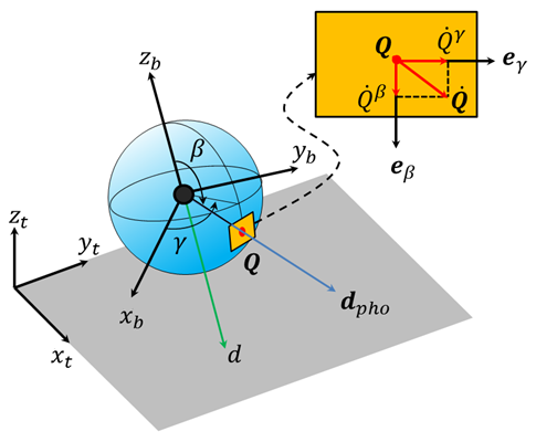 | Figure 1. Spherical Image Model for WFI of optic flow |
The optic flow  is expressed with two components along the azimuth and elevation directions, i.e.,
 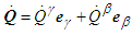 where
where  is a unit vector. The components are
 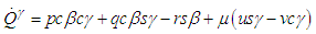 | (3) |
 | (4) |
where  and
and  Note that since optic flow is measured in the image surface of two-dimension, the depth component is zero. Furthermore, when the terrain surface is modelled as a flat, infinite, and horizontal plane, the nearness function
  can be expressed as follows:
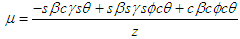 | (5) |
where  and
and  are the roll and pitch angles of the vehicle expressed in the 3-2-1 Euler angle sequence. Note the yaw angle
  does not appear in Eq. (5), because the flat-plane assumption makes no difference on optic flow for any yaw angle.
2.2. Wide-Field-Integration of Optic Flow
The output of WFI of optic flow is obtained from an integration of optic flow and “sensitivity function” over the space S2. For the j-th sensitivity function defined as | (6) |
the corresponding output is calculated from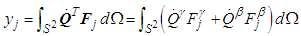 | (7) |
where  is a solid angle on the spherical image surface. For three-dimensional motion estimations, spherical harmonics are frequently used as the sensitivity functions, while Fourier series are often used for two-dimensional cases.The concept of sensitivity functions was introduced in Humbert [3]. However, the meaning of those functions was not uniquely defined from physical viewpoints of sensors or vehicles. Furthermore, the space integration shown in Eq. (7) requires large computational load, and thus it is not realistic for microprocessors to perform the calculations in a short time interval. Thus, the method using Riemann sum was proposed in Ref. [12] instead of the space integration as a practical evaluation method. Furthermore, the following should be noted for the WFI of optic flow. As shown in Eq. (2), optic flow is a function of the nearness function
  to a point on the terrain. This means that optic flow obtained by onboard sensors is different according to terrain surface profiles even in a same vehicle motion. However, when the optic flow is integrated (or summed) over a wide region, the effect of each nearness function caused by uneven terrains is averaged in the integration process. That is, the output yj obtained for uneven terrains approaches to that for a flat terrain according to the extent of integration regions, when the terrains are randomly rough.
2.3. Motion Estimation from WFI of Optic Flow
After the replacement with the Riemann sum, Equation (7) becomes an algebraic relation. Then, when the attitude and altitude are measured by other sensors, the output yj can be evaluated in two ways: one utilizes optic flow obtained with sensors boarded on a vehicle, while another utilizes optic flow mathematically evaluated from Eqs. (3)-(5) under the flat-surface assumption for the specified attitude and altitude.Generally, the motion variables of a vehicle are composed of the vehicle’s position (x, y, z), velocity (u, v, w), attitude angle  and angular rate (p, q, r). However, when the WFI of optic flow adopts the flat-surface assumption, the variables x, y, and
  do not appear in the relation because they do not generate any difference to optic flow. Furthermore, although the vehicle’s attitude angles
  and altitude variables
  appear in nonlinear form in Eqs. (3)-(5), the remained motion variables are linear in these equations. Thus, when the attitude angles
  and the altitude z are measured with other sensors in the standard WFI of optic flow procedure, the output of WFI of optic flow, Eq. (7), has a linear relation with the following 6-state variables:
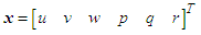 | (8) |
Thus, by using the optic flow obtained at discrete photoreceptors, the output vector corresponding up to the M-th sensitivity functions can be expressed as follows: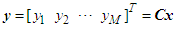 | (9) |
where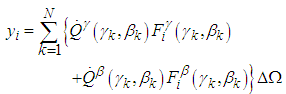 | (10) |
N indicates the total number of photoreceptors, and C is the coefficients matrix of the 6-state variables. The elements of the matrix C can be mathematically calculated from Eqs. (3)-(5) and (10). Note that since the number of photoreceptors is sufficiently larger than 6 of the estimated state variables, the matrix C should have full rank obviously. Thus, by using the pseudo inverse matrix  the state variables x can be estimated as follows.
 | (11) |
3. Effect on Estimation Accuracy
This section first discusses the accuracy of the motion estimation considering the relation of optic flow components and the sensitivity function shown in Eq. (6). Then, the effects of the restrictions of real image sensors on the estimation accuracy are examined to improve the accuracy in the WFI of optic flow processing.
3.1. Sensitivity Functions
This paper reconsiders the expression and its meaning of the sensitivity functions used in the Refs. [8-10]. For the vector form sensitivity function shown in Eq. (6), the output is expressed as Eq. (7) for rigours space integration or as Eq. (10) for discretised form. These expressions, however, indicate that the azimuth and elevation components are treated equivalently and combined. As such, only a combined signal is used for the states estimation, although they are two different signals. Hence, to deal with each component as a different signal, the following form of sensitivity should be used instead of Eq. (6).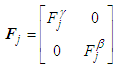 | (12) |
Then Eq. (7) is replaced with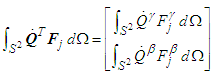 | (13) |
Consequently, the WFI of optic flow outputs having  components for up to the M-th sensitivity functions are expressed by using the Riemann sum as follows:
 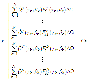 | (14) |
To examine the effect of the new form of the sensitivity functions, computer simulations have been conducted by using a level flight shown in Table 1 as an example. Since the estimation accuracy of WFI of optic flow is also dependent on other parameters of the image sensor, the following conditions are used in the simulation: A camera is facing  -axis, its field of view is defined as
 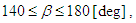 and the photoreceptors are placed every two degrees in both the azimuth and elevation directions (i.e., the number of photoreceptors N is 3,600). Furthermore, as a model of sensor noises for optic flow, it is assumed that each component of optic flow is contaminated with white noise with zero mean value and standard deviation of 0.3 [rad/s], while the altitude of a vehicle is assumed to be accurate. (The errors of attitude sensors are explained in the next subsection).
Table 1. Level Flight Condition of a Vehicle used in Simulations
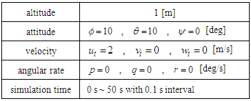 |
| |
|
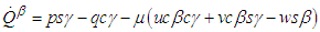
The estimated results are shown in Figure 2. The red line indicate the result by using the proposed form of the sensitivity functions, the blue one is by using the conventional form of sensitivity functions, and the black line shows true variable. The standard deviations of the estimated motion variables are compared in Figure 3. These results clearly indicate the superiority of the proposed form of sensitivity functions, Eq. (12). Especially, the estimation accuracy of w and r is highly improved. This is because that these variables are included in one component of optic flow as shown in Eqs. (3) and (4). Thus in the proposed form, another equation is free from the noises of these variables.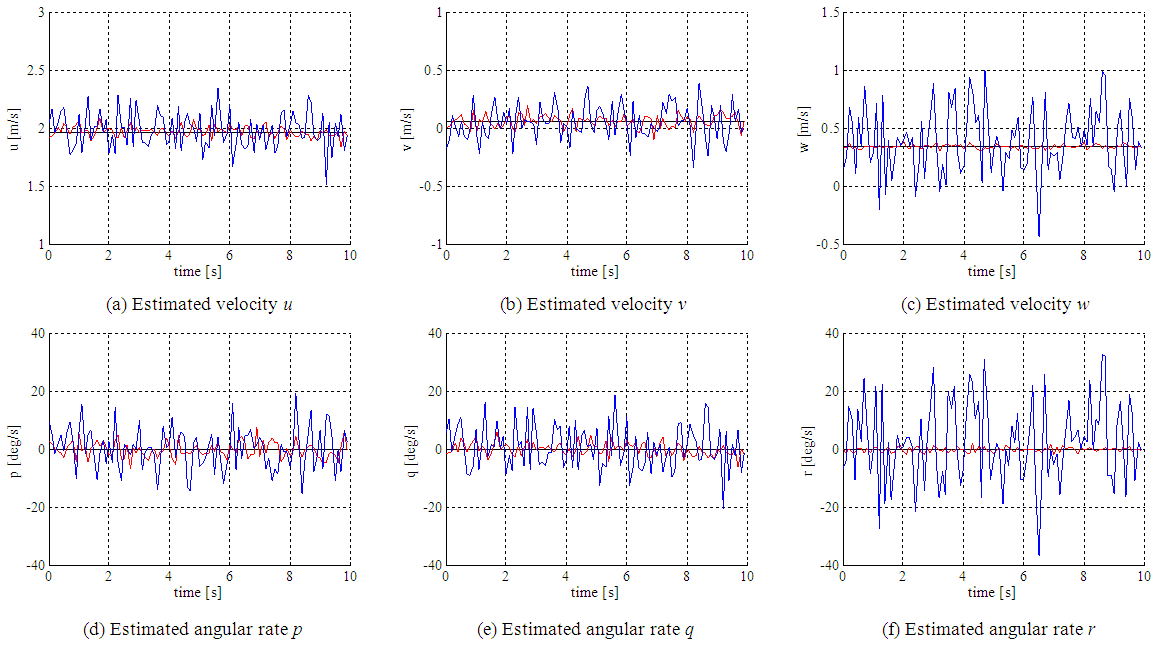 | Figure 2. Motion variables estimated by different sensitivity functions (  proposed one, proposed one,  conventional one, conventional one,  true value) true value) |
 | Figure 3. Comparison of the standard deviations of the estimated motion variables for different sensitivity functions |
This superiority can be analytically explained as follows by considering noises included in optic flow. Optic flow data contaminated with the noises are expressed as | (15) |
where  is a random noise vector in the azimuth or elevation directions, respectively. Assume the noises’ mean values are zero, and their variances are
  and
and  respectively. Then, for the conventional form of sensitivity functions, the observation noise included in the WFI of optic flow output is expressed as
 | (16) |
where  denotes the inner product including the effect of space integration for discretized data, and
 Then, the (i,j)-component of the covariance matrix is
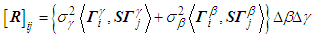 | (17) |
where 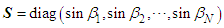 . When spherical harmonics are used as sensitivity functions, since
 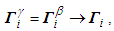 the (i,j)- component is evaluated as follows.
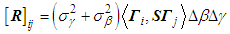 | (18) |
On the other hand, for the proposed form of sensitivity functions, the observation noise aligned as the sensor output (15) is expressed as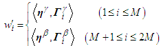 | (19) |
Then the (i,j)-component of the  covariance matrix is
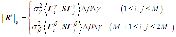 | (20) |
Note that since noises are no correlation,  for
for  and
and  or vice versa. Equations (17) and (20) indicate that the proposed form has larger data number and smaller covariance of noises than those of conventional form. Thus, the effect of sensor noises becomes smaller in the proposed form than the conventional one.
3.2. Effects of Practical Restrictions of Image Sensors
In the standard WFI of optic flow theory used in [8-11], photoreceptors are assumed to be placed on a whole spherical surface and measure optic flow. However, in practical systems, optic flow is obtained through computer vision processing for standard camera images. This implies that optic flow obtained by real sensors has restrictions for its region and number / distribution of photoreceptors. In this subsection, the effects of the practical restrictions are examined in numerical simulations considering optic flow noises. Furthermore, although two types of sensor signals (attitude and altitude information) are appeared in Eqs. (3)-(5), here only the effect of the attitude sensor noises is investigated due to the following reason. From Eqs. (2) and (5), when all of the vehicle’s angular rates are closed to zero, the altitude sensor error linearly changes the optic flow. Thus, the effect of altitude sensor noises can be roughly anticipated from the effect of optic flow noises, while attitude sensor errors influence to optic flow nonlinearly. In the simulations shown below, as an example, white noises with zero mean value and 4 degrees of standard deviation are added to the optic flow and the attitude sensor output. Furthermore, to specify the effect of vehicle’s flight modes, this paper shows the result for a vertical descent condition shown in Table 2 as well as the level flight in Table 1.Table 2. Vertical Descent Motion used in Simulations
 |
| |
|
(a) Effect of optic flow regionFor simplicity, the optic flow region to be integrated is characterized as follows. A standard image sensor facing to  -axis is used and its field of view is specified with the elevation angle
  although a camera’s field of view is usually defined as a rectangle. In the evaluations, three regions of optic flow are compared:
  [deg],
  [deg], and
  [deg]. To unify other parameters, the number of optic flow is set as
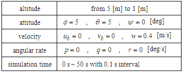
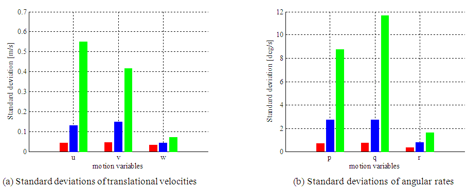
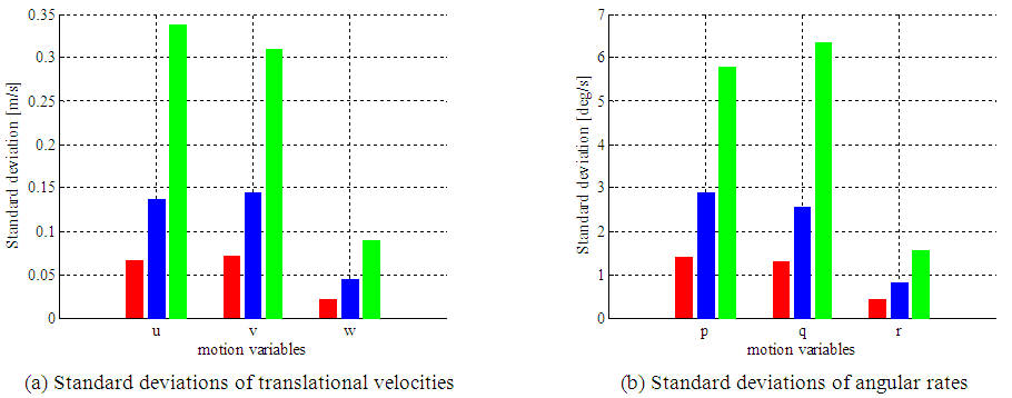
  and their distribution is assumed to be uniform in both the elevation and azimuth directions.The results are shown in Figures 4-7. In each figure, (a) indicates the standard deviations for the estimated translation velocities, while (b) is those for the angular rates. The red, blue, and green bars correspond to the large (
 [deg]), the medium (
 [deg]), and the small (
 [deg]) ranges, respectively. Figures 4 and 5 are results considering the optic flow noises specified above, and Figures 6 and 7 are for the attitude sensor noises. Furthermore, Figures 4 and 6 indicate the results in the level flight, while the results of the vertical descent are shown in Figures 5 and 7.
 | Figure 4. Comparison of the standard deviations of the estimated motion variables for different integration regions w.r.t. optic flow noises in a level flight.  |
 | Figure 5. Comparison of the standard deviations of the estimated motion variables for different integration regions w.r.t. optic flow noises in a vertical descent.  |
 | Figure 6. Comparison of the standard deviations of the estimated motion variables for different integration regions w.r.t. attitude sensor noises in a level flight.  |
 | Figure 7. Comparison of the standard deviations of the estimated motion variables for different integration regions w.r.t. attitude sensor noises in a vertical descent.  |
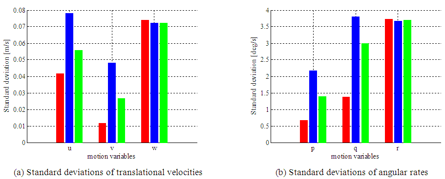
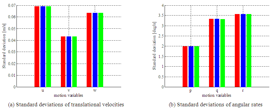
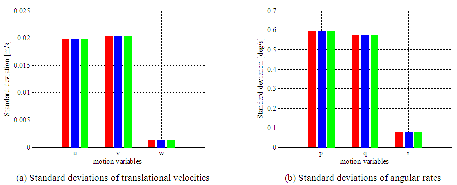
From Figures 4 and 5, for optical sensor noises, the superiority of the large integration region is obvious even when the number of optic flow vectors is same, regardless the flight modes. Since optic flow noises are inevitable, this result suggests that an image sensor with a wider field of view is desirable. However, for attitude sensor noises, apparent tendency for integrated regions are not seen in Figures 6 and 7. Thus, attitude sensors with better accuracies are desirable in the application of WFI of optic flow. Furthermore, the comparison between Figures 6 and 7 indicates the relations between vehicle’s moving directions and estimation accuracy. In the level flight (ut=2 [m/s], vt=wt=0 [m/s]), Figure 6 shows that the estimation accuracies of the variables relating to xb- and yb-axes become better than that to zb-axis, whereas Figure 7 for the vertical descent clearly indicates better estimation accuracy for zb-axis related variables. (b) Effect of the number of optic flowFigures 8 to 11 indicate the estimation accuracy for the number of optic flow integrated in the estimation process under a specified field of view. The same as above, in each figure, (a) and (b) indicate the standard deviations for the estimated translational and rotational velocities. The red, blue, and green bars correspond to the large number of optic flow (N=14,400), the medium one (N=3,600), and the small one (N=900), respectively for the same region defined by  [deg]. Since the optic flow is assumed to be obtained in same intervals in the elevation and azimuth directions, the red, blue, and green mean to use optic flow obtained for
  [deg],
  [deg], and
  [deg], respectively. Figures 8 and 9 are results considering the optic flow noises, and Figures 10 and 11 are for the attitude sensor noises. Figures 8 and 10 indicate the results in the level flight, while the results of the vertical descent are shown in Figures 9 and 11.For the case of optical sensor noises, Figures 8 and 9 imply that the denser optic flow integration clearly gives much better estimation accuracy in any flight modes. However, for altitude sensor noises, the number of optic flow has no effect on the estimation accuracy as shown in Figures 10 and 11. The dependency between a vehicle’s moving direction and the estimation accuracy are still seen in Figure 11, but it is less clear in Figure 10.
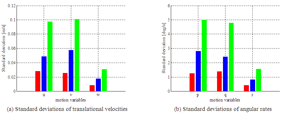 | Figure 8. Comparison of the standard deviations of the estimated motion variables for different resolutions w.r.t. optic flow noises in a level flight.  |
 | Figure 9. Comparison of the standard deviations of the estimated motion variables for different resolutions w.r.t. optic flow noises in a vertical descent.  |
 | Figure 10. Comparison of the standard deviations of the estimated motion variables for different resolutions w.r.t. attitude sensor noises in a level flight.  |
 | Figure 11. Comparison of the standard deviations of the estimated motion variables for different resolutions w.r.t. attitude sensor noises in a vertical descent.  |
(c) Effect of the distribution pattern of optic flowHere, three distribution pattern of optic flow is examined under the following conditions; the optic flow region for integration is specified by  [deg], and the number of optic flow is set as N=3,600. In the first pattern, optic flow is assumed to be obtained at
  the second and third patterns use
  ,
,  and
and  respectively. The standard deviations are shown in Figure 12 for a case with optic flow noises in the level flight shown in Table 1. This result indicates the distribution pattern of optic flow has little effect on the estimation accuracy.
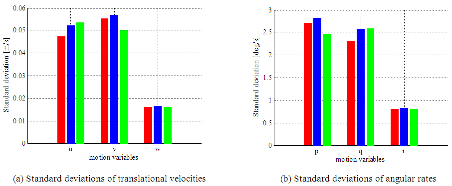 | Figure 12. Comparison of the standard deviations of the estimated motion variables for different distribution patterns of photoreceptors w.r.t. optic flow noises in a level flight.     |
Through the three examinations shown above, the desirable features of real sensors used in WFI of optic flow can be summarized as follows: Image sensors with a wide field of view and high resolution are desirable. When such desirable image sensors are applicable, the errors of altitude sensor outputs are not so critical because the effect can be alleviated. While for attitude sensors, high accuracy sensors are strictly desirable for better motion estimation.
4. Verification in Experiments
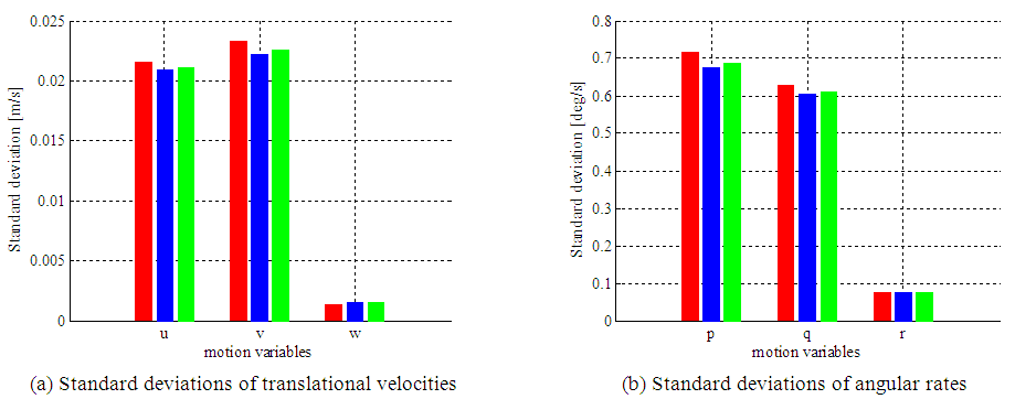
To verify the effectiveness of the proposed form of sensitivity functions shown in Eq. (12), experiments have been conducted for several conditions. Figure 13 shows the optic flow sensor used in the experiments. The sensor is OpticalFlow-Z made by ZMP Inc., and its processing algorithm has been improved to generate 79 59 optic flow vectors for the field of view 45.1 [deg] 34.6 [deg] with a frame rate of 10 [fps].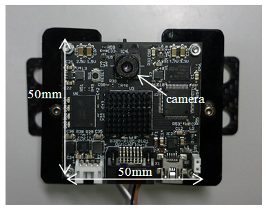 | Figure 13. Optic flow sensor used in experiments |
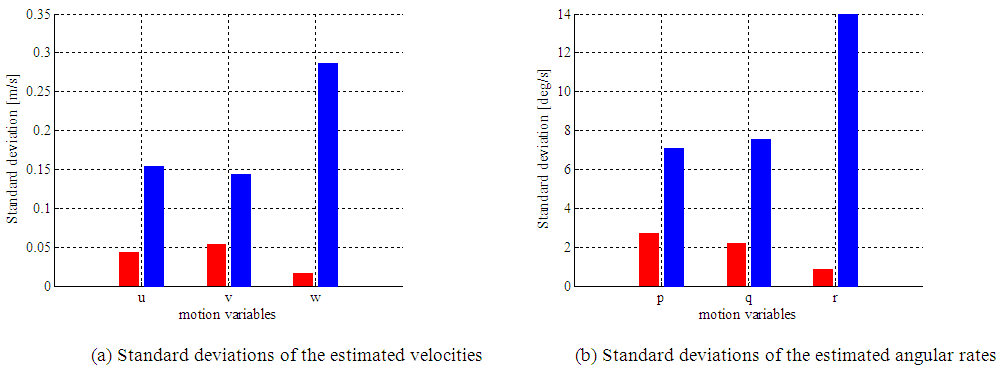
Figure 14 shows a typical result for an estimated velocity component: red line indicates the result by the proposed form of sensitivity functions, while blue one is the estimation by the conventional form. To verify the reliability of the results, the associated velocity component calculated from the data of a motion capture sensor with millimeter-accuracy in 50 Hz is also shown in black. Apparently, the proposed form of sensitivity functions shows much better coincidence with the motion capture result. Assuming the motion capture result is true, the standard deviations of the proposed and standard form of sensitivity functions are compared in Figure 15. These results indicate the effectiveness of the proposed form, Eq. (12).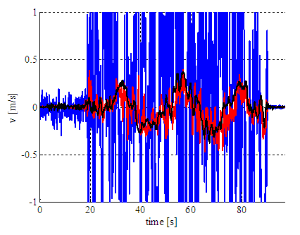 | Figure 14. Comparison of an estimated velocity component by different methods ( proposed form of sensitivity functions, proposed form of sensitivity functions,  standard form of sensitivity function, standard form of sensitivity function,  motion capture sensor) motion capture sensor) |
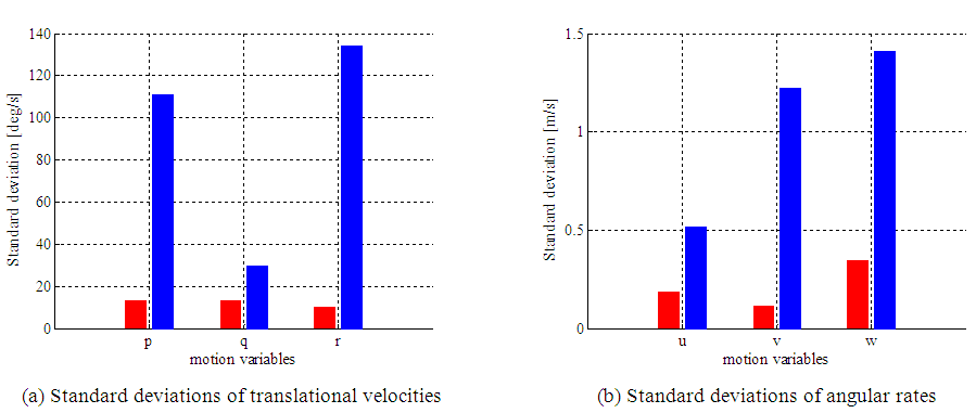 | Figure 15. Comparison of the standard deviations for the proposed and standard form of sensitivity functions in experiments. ( proposed form of sensitivity functions, proposed form of sensitivity functions,  standard form of sensitivity functions) standard form of sensitivity functions) |
5. Conclusions
This paper, first, has re-examined the form of sensitivity functions used in the WFI of optic flow, considering the relation of optic flow components and the sensitivity function. Then, considering the application of WFI of optic flow with a practical image sensor, the effects of the restrictions (the integration region, the number, and the distribution pattern of optic flow) have been examined in numerical simulations. Finally, through some experiments, the effectiveness of the proposed form of sensitivity functions has been verified.
ACKNOWLEDGEMENTS
The research is supported by Japan Society for the Promotion of Science (JSPS) KAKENHI Grant-in-Aid for Challenging Exploratory Research No. 15K14254.
References
| [1] | Koenderink J. J. and van Doorn A. J.: Facts on Optic Flow, Journal of Biological Cybernetics, 56 (1987), pp.247-254. |
| [2] | Egelhaaf, M., Kern, R., Krapp, H. G., Kretzberg, J., Kurtz, R. and Warzecha, A.: Neural encoding of behaviourally relevant visualmotion information in the fly, Trends in Neurosciences., 25 (2002), pp. 96-102. |
| [3] | Humbert, J. S., 2006, Bio-Inspired Visuomotor Convergence in Navigation and Flight Control Systems, Ph.D. Dissertation, Mechanical Engineering, Department, California Inst. of Technology, Pasadena, CA. |
| [4] | Humbert J. S., Murray R. M. and Dickinson M. H.: A Control-Oriented Analysis of Bio-inspired Visuomotor Convergence, Proceedings of the IEEE Conference on Decision and Control, 2005, pp. 245-250. |
| [5] | Humbert J. S. and Frye M. A.: Extracting Behaviorally Relevant Retinal Image Motion Cues via Wide-Field Integration, Proceedings of the American Control Conference, 2007, pp.2724-2729. |
| [6] | Epstein M., Waydo S., et al.: Biologically Inspired Feedback Design for Drosophila Flight, Proceedings of the American Control Conference, 2007, pp.3395-3401. |
| [7] | Conroy, J., Gremillion, G., Ranganathan, B. and Humbert, J. S.: Implementation of Wide-Field Integration of Optic Flow for Autonomous Quadrotor Navigation, Autonomous Robots. 27, No. 3 (2009), pp. 189-198. |
| [8] | Hyslop, A. M., and Humbert, J. S., 2010, Autonomous Navigation in Three-Dimensional Urban Environments Using Wide-Field Integration of Optic Flow, Journal of Guidance, Control, and Dynamics, Vol. 33, No. 1, pp. 147–159. |
| [9] | Hyslop A. M., Krapp H. G. and Humbert J. S.: Control theoretic interpretation of directional motion preferences in optic flow processing interneurous, Journal of Biological Cybernetics, 103 (2010), pp.353-364. |
| [10] | Shoemaker M. A. and Hokamoto S.: Application of Wide-Field Integration of Optic Flow to Proximity Operations and Landing for Space Exploration Missions, Advances in the Astronautical Sciences, 142 (2011), pp.23-36. |
| [11] | Izzo, D., Weiss, N. and Seidl, T.: Constant-Optic-Flow Lunar Landing: Optimality and Guidance, Journal of Guidance, Control, and Dynamics., 34, No. 5 (2011), pp. 1383-1395. |
| [12] | Shoemaker, M. A. and Hokamoto, S., 2013, Comparison of Integrated and Non-integrated Wide-Field Optic Flow for Vehicle Navigation, Journal of Guidance, Control, and Dynamics, Vol. 36, No.3, pp.710-720. |

 Abstract
 Reference
 Full-Text PDF
 Full-text HTML