1. Introduction

Since multi-legged robots can operate under extreme conditions where it would be difficult for humans to work, a wide variety of research has been carried out on topics related to six-legged robots, which can walk with a duty factor of 0.5 while maintaining static stability [1, 2]. There has been much research on six-legged robots related to the development of sensor technology. For example, self -localization using global position satellite system (GPS) sensors [3], autonomous walking control in an obstacle space by using laser rangefinders (LRFs) [4], recognition of a walking environment by using stereo cameras [5], walking control to follow a target object by using RGB-D sensors [6], and classification and recognition methods for walking surfaces [7, 8]. With the abovementioned technological advances, a control technology to realize more highly precise work is required for the practical use of the multi-legged robots. Unlike manipulators, legged robots move their position to support their body by continuous walking, so it is generally difficult to increase the accuracy in work using a legged robot. Previous studies have reported methods for correcting deviations from a target walking trajectory [9, 10], and methods for correcting the position of the center of gravity (CoG) of a robot body, as well as its yaw angle [11, 12]. The problem of precise movement becomes more complicated in the case of a multi-legged robot walking on rough terrain. In this case, posture control is necessary [13]. Biological methods for the posture control of a six-legged robot have been reported [14-16], and there are also reports dealing with posture control methods from the viewpoint of the model base of the robot [17-19]. Further, a report has been made on a six-degree-of-freedom (6-DoF) control of the body of a wheeled robot with four legs [20]. However, we are unable to find reports dealing with 6-DoF control of the body of a six-legged robot from the viewpoint of a model base.

In this paper, we discuss a 6-DoF control method that controls posture, body position, and yaw angle using a six-legged robot equipped with a leg mechanism proposed by Hirose et al. [21]. Figure 1 shows a model of one of the legs. Each leg has 4-DoF, which are provided by a rotating link , a thigh link , a shank link , and a foot sole . First, we describe the previously used posture control method [19]. Next, we describe our proposed walking directional control. The six-legged robot used in this study has three joints, which are driven by actuators at the rotating, thigh, and shank links. In our previous study [12], a walking directional control method in which the only control inputs were the rotating link torques was described. More specifically, when walking with three-legged support, the reaction force from the support legs becomes a propulsive force acting on the body. Accordingly, in this situation, we can derive a mathematical model in which the torque of rotating links and reaction forces of thigh and shank links are control inputs for controlling the body position and yaw angle. To explore our posture control and walking directional control models, we built a Type-1 servo system and designed a linear-quadratic-integral (LQI) control system that permits the robot to follow the target trajectories of body posture, body position, and yaw angle. One problem encountered at this point is that the FB inputs for the thigh and shank links generated by the walking directional control interfere with the FB input for the thigh link generated by the posture control. Herein, we will explain how the FB control input by our posture control method generates a control input that eliminates the interference produced by the walking directional control. More specifically, the FB inputs acquired by the LQI control system in the walking directional control are converted into correction amounts for the target angles of the rotating and shank links of the support legs, which allows the target trajectories of the rotating and shank links to be corrected. The effectiveness of this proposed method is confirmed through simulations using a 3D model of the six-legged robot.

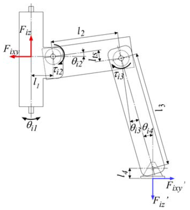Figure 1. Model of one leg of a six-legged robot

2. Six-legged Robot and 3D CAD Model

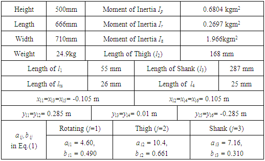
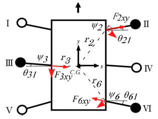
Figure 2 shows the six-legged robot used in this study, the specifications of which are shown in Table 1. In this leg mechanism design, the velocity of the robot’s body is generated by the rotating link, while the body weight is supported by the thigh link. Note that this design permits the shank to move in directions that would be difficult for a rotating link to replicate. Each leg link except for is driven by a worm gear. The self-locking function of the worm gear cancels the body weight torque in the thigh link. is a passive rotational joint, and the range of movement is . 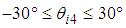Figure 1 shows the relationship between the forces and the reaction forces working at the rotating axis. are forces working in the horizontal and vertical directions at the sole of the support leg, respectively. is the sum of , and . shows the fluctuation of the horizontal force caused by slippage and model error. is the sum of and . shows the vertical force fluctuation of the model error. Robot motion is driven by the control input, which requires current flow from the motor driver to the motor through a digital-to-analog (D/A) converter. The body of the robot is equipped with an LRF, a posture sensor that detects the pitch and roll angles of the body, and an ultrasonic sensor that detects the body height. Figure 3 shows a 3D computer-aided drafting (CAD) model of the six-legged robot shown in Fig. 2. The model was created by connecting a total of 19 elements (one body, three leg joints) using revolute joints. Each revolute joint in the 3D CAD model has a frequency response in the actual robot (Fig. 2), which can be approximated using the following second-order transfer function:

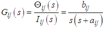(1)

Here, represents the leg link rotation angle, represents the command current to the motor driver, i represents the leg number (1 to 6), and j represents the rotating link (1), the thigh link (2), or the shank link (3). Table 1 shows the and values for the rotating link, thigh link, and shank link. In addition, four contact points are present on the underside of the foot at the end of each leg, and contact with the walking surface is modeled using springs and dampers . The coefficient of friction (CoF) is taken to be 0.35. In this study, the robot is modeled in 3D using Virtual. Lab Motion (Siemens PLM Software, Plano, TX), and numerical calculations are carried out using MATLAB®/Simulink (MathWorks, Natick, MA). The nonlinear equation of motion for the robot is derived automatically in Virtual.Lab Motion. Furthermore, the actual robot mechanism is designed so that the shank and the foot underside are connected by a revolute joint, and the entire foot underside makes contact with the walking surface. However, this revolute joint is not included in the 3D CAD model. The error influence caused by the absence of this revolute joint in the model is reduced by designing the walking trajectory as follows: (1) the trajectory is set in a way that ensures that the shank is always roughly perpendicular to the walking surface, and (2) the walking speed is set in a way that ensures that the influence of supporting leg slippage in the 3D simulation is small. This assumes stable operation/walking on uneven terrain. In the simulation, the maximum slip velocity in the x and y directions is 0.002 m/s, and approximately 0.01 m of slippage occurs in the 5-s support phase. Since the control method used in this study is affected by the reaction forces acting on the support legs, it is preferable that no slippage occur. However, since it is impossible to create a walking environment in which there is absolutely no slippage, the effectiveness of the control method is tested in a walking environment where slippage occurs in the support legs. Furthermore, the model error produced by can be considered as the fluctuation of shown in Section 4.3.

Table 1. Specifications of six-legged robot

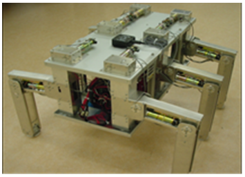Figure 2. Six-legged robot

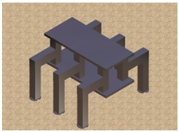Figure 3. 3D CAD model of six-legged robot

3. Walking Planning

Figure 4 shows the leg numbers of the six-legged robot and Fig. 5 shows the gait pattern produced by the three support legs. From these figures, it can be seen that static stability is maintained because the body CoG projection to the walking surface is certain to remain within the polygon created by the support legs. In this study, since it is assumed that the robot walks on uneven terrain, we will examine the walking control method in order to evaluate its ability to control the robot posture and follow the set trajectory. In view of the actuator responsiveness, the orbit of the six-legged robot is set at 10 cm per step and T, the walking cycle period, is set at 10 s. The sole of each leg was made to rise 5.5 cm above the walking surface during its swinging phase. The reference signals of the joint angles are calculated by using inverse kinematics from the toe orbit. In this study, the six-legged robot walks using three support legs and three swinging legs.

Figure 4. Walking patterns

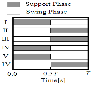Figure 5. Walking patterns

4. 6-DoF Control Method

4.1. Posture Control

4.1.1. Posture Model of Six-Legged Robot

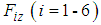
As shown in Fig. 4, the six-legged robot is supported by three legs (Legs I, IV, and V). Here, the force in the vertical direction of the support leg is , the mass of the body is , the inertia around the pitch and roll axes are and , respectively, the body height is , the pitch and roll angles of the body are and , respectively, and the coordinates of the rotating link between the body and the shoulder at the support legs are 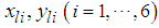. The motion equations of the force and moment equilibrium in the vertical direction and those for the pitch and roll axes in supporting the six-legged robot by three legs are shown as Eq. (2) [19]. Here, the deviation of the rotating angles is assumed to be small. The subscripts (2), (3), and (6) denote the support legs that are designated Legs II, III, and VI, respectively.

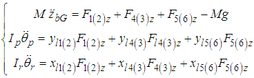(2)

4.1.2. Thigh Link Model Setting the Virtual Impedance

In this section, we consider a situation in which the robot body is supported statically in the case of applying the feedforward (FF) force obtained by Jacobian or counterbalancing the load of the body mechanically. FB control provides the posture control needed to control walking posture variations. In this study, the imaginary force and moments controlling the desired posture are generated at the rotating link of the thigh shown in Fig. 6, as the reaction force of the force acting on a support leg. This imaginary force and these moments are shown as in Eq. (2).

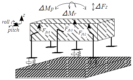Figure 6. Imaginary impedance model of FB control for a six-legged robot

In this situation, the imaginary force, which is the reaction force acting on the rotating thigh link (which is also acting on the tip of the support leg in the vertical direction), is modeled by using a spring and a damper, as shown as Fig. 7. This figure shows the relationship of the leg links generating the reaction force at the thigh link by using the imaginary spring and damper in a situation where the six-legged robot body is kept stable by statically applying FF control inputs. In Fig. 7, is the thigh length, and changes due to changes in and . It is assumed that the variation effects are small, and is approximated as . Additionally, and are respectively the damping and spring coefficients used to generate the imaginary force shown as Eq. (3-a). In this figure, it is assumed that the shank always becomes vertical to the ground 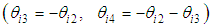. Based on that assumption, the FB force generating the imaginary force and moments leads to the following Eqs. (3-a) and (3-b). Moreover, the angles of the thigh are not permanently at zero degrees on irregular terrain, such as on a step. shows the deviation on the irregular terrain. Figure 8 shows the relation of the displacement difference between and . In Fig. 8, the red dashed line shows the relation between the body and the thigh link in the case of . The imaginary force acting on the support leg by the imaginary impedance is shown as follows:

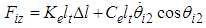(3-a)

(3-b)

Here, it should be noted that the thigh link range of movement used in this study is –30° to +30°, and the mechanical feature is that supports the weight of the robot body by the thigh link, is linearized at zero degrees as follows:

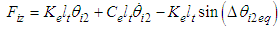(4)

Next, the force acting in Eq. (4) acts as a load torque on the thigh link in order to realize the desired body posture. In this study, a direct current (DC) motor drives the thigh link and the current controls the DC motor. The equilibrium equation of the FB torque is Eq. (5) for the thigh link, as shown in Fig. 7. Here, we consider the fluctuation of the vertical force

(5)

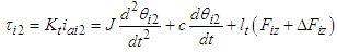
where is the armature current of the DC motor, is the angle between the body and thigh, is the torque constant, is the moment of inertia, and is the mechanical viscous damping coefficient. In Eq. (5), 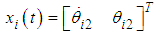, , and the state equation and the output equation from current to the DC motor are expressed as

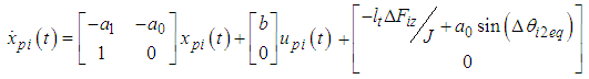(6-a)

(6-b)

where

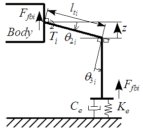Figure 7. Relationship between the thigh angle and the imaginary force in the vertical direction of the support leg

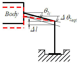Figure 8. Relationship between and

4.1.3. FB Posture Model of Six-Legged Robot

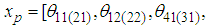
By substituting Eq. (5), which is each force in the case of setting the imaginary impedance, for Eq. (2), and defining the 12th-order state value , which comprises the state values of each thigh link, the pitch and roll angles, the body height, and the velocity, the following state equation is obtained. The body height is zero in the case of . Subscripts (2), (3), and (6) denote the support legs (Legs II, III, and VI, respectively).

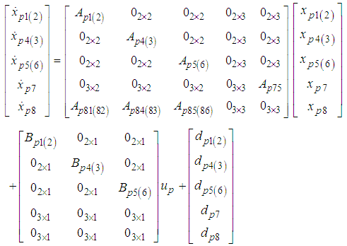(7)

where

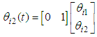
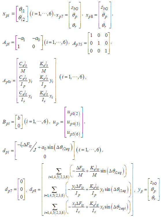Then, Eq. (7) can be rewritten to give the following output equations:

(8-a)

(8-b)

4.2. Walking Directional Control Model

Figure 9 shows the relationship between the torques generated by the rotating links with three-legged support and the forces acting on the body as a result of these reaction forces. Figure 10 shows the relationship between torques generated by the thigh and the shank links with three-legged support and the forces acting on the body as a result of these reaction forces. Here, represents the direction of travel in the robot coordinate system, represents the horizontal direction perpendicular to the -axis, and represents the yaw angle of the body of the robot's body, which is the angle of rotation about the -axis. represents the mass of the robot’s body, is the moment of inertia about the -axis, and is the angle of the revolute joint in the rotating link. For , the clockwise direction is taken as positive, while for , the counterclockwise direction is taken as positive. 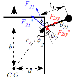represents the position vector from the CoG of the robot's body to the rotational center of the rotating link of each leg. Figure 11 shows the relationship between the forces acting on Leg II (a support leg), and the forces , which are the components of that act perpendicular to . 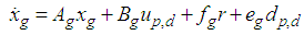indicates the angle between and . The equations of motion for the CoG of the robot's body in the x-direction, y-direction, and about the yaw angle (which are derived in the same way for the situation where Legs I, IV, and V are the support legs) are

(9)

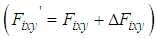
where , , and are the total fluctuations of the force in the x-direction, the force in the y-direction, and the moment about the -axis, respectively. Here, defining the state variable vector as and the control input vector as 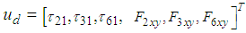, gives the following state and output equations:

(10-a)

(10-b)

where

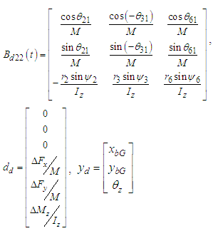The input matrix is time-variant. Here, considering the range of movement , in given in Eq. (10) is fixed as follows. are set to . When are positive, , and when , . In addition, . In this study, the FB control system is designed by as a time-invariant matrix.

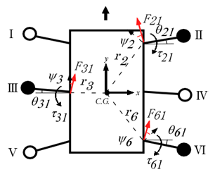Figure 9. Reaction forces at the body received from the rotating links

Figure 10. Reaction forces at the body received from torques generated by the thigh and shank

Figure 11. Relation among φ, θ, and ψ

4.3. Optimal Servo System

The servo system used to suppress the effect of the disturbance is designed by considering the FB models shown in Section 4.1.3 and Section 4.2. Because body posture step references and step disturbances seem to occur frequently in an environment where the robot is active, a Type-1 servo system was designed:

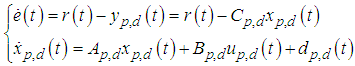(11)

where the matrixes and vectors in Eq. (11) correspond to those in Eq. (8) and Eq. (10). is the error vector between the desired vector and the output vector . Describing Eq. (11) as a matrix, we obtain the following:

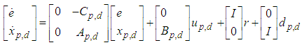(12)

Further, Eq. (12) can be rewritten as the following equation:

(13)

The control input is obtained to minimize the following equation:

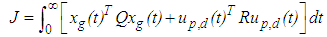(14)

Here, and are weighting matrices given by the design specifications, where . The control input used to minimize Eq. (14) is given by the following equation:

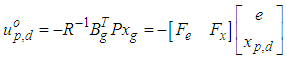(15)

Here, is the unique positive definite solution of the following Riccati equation:

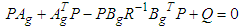(16)

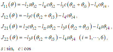
The FB control input of the thigh link by the posture control is the current in Eq. (5). In addition, the FB control inputs by the walking directional control are for the rotating link and the reaction force for the thigh and shank links.

The relationship between the thigh and shank torques and the body reaction forces from the support legs is expressed by the Jacobian matrix in the leg mechanism, as shown in Fig. 2. The relationship between , , and forces , acting at the sole of the support leg is shown as follows:

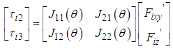(17)

where

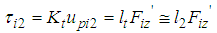
Here, we consider FB control input of the thigh link. in Eq. (17) is shown as follows:

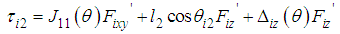(18)

where

With the approximation , Eq. (18) can be rewritten by the following equation:

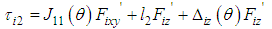(19)

The static relationship in Eq. (5) is shown by the following equation:

(20)

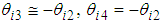
By comparing Eq. (20) with Eq. (19), it can be seen that the terms of the FB control input by the walking directional control and of the model error , including the rotating link , become the disturbance input interfering with the FB control input of the posture control. The control input of the shank is shown as follows:

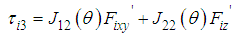(21)

Here, using the approximations , is approximated by . is dominated by the term. Therefore, in this study, is obtained by multiplying by .

5. 3D Simulations

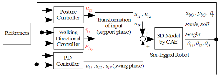
Figure 12 shows a block diagram of the 3D simulation conducted in MATLAB/Simulink. In this simulation, the robot walks in a straight line. In Fig. 11, the FB control inputs of the posture control and the walking directional control are transformed to , and , which are control inputs for the rotating, thigh, and shank links, respectively. Figure 13 shows a block diagram of the transformation part of the control input for one support leg. The rotating and shank links are primarily controlled by the walking directional control. In the walking directional control, steady-state deviation occurs in the type-1 servo system because the reference signals of the robot change with time. Thus, we can see that the controlling state of the rotating and thigh links used by the proportional derivative (PD) control to follow the reference signals is a steady state. In this study, when the control performance degrades due to walking disturbance, a walking directional controller is used to decrease the walking disturbance effect. The FB control inputs and produced by the walking directional control are converted into modified reference signal amounts by coefficients , , and . The PD control for each leg link in Fig. 11 is given by the following equation:

(22)

Figure 12. Block diagram of control system

Table 2. Simulation parameters

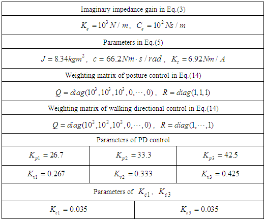
Here, i = 1 to 6 (leg numbers), j = 1 (rotating link), 2 (thigh link), or 3 (shank link), indicates the proportional gain, and is the velocity gain. The FB control input can also be converted as a modified thigh amount, but inputs directly into the thigh in this study. Table 2 shows the parameters used in our 3D simulations. An interval of 1 s, when the three support legs switch to the swinging phase after the three swinging legs land firmly on the ground, is set as the switching length of the support legs to stabilize the posture. Additionally, in order to more clearly examine the input interference of walking directional control on the posture control input, the influence of the interference was increased to , as shown in Fig. 12.

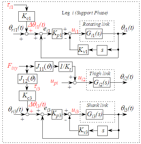Figure 13. Block diagram of one leg in support phase

5.1. Walking on Even Terrain

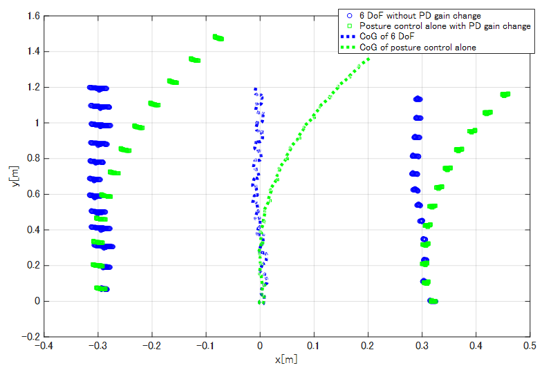
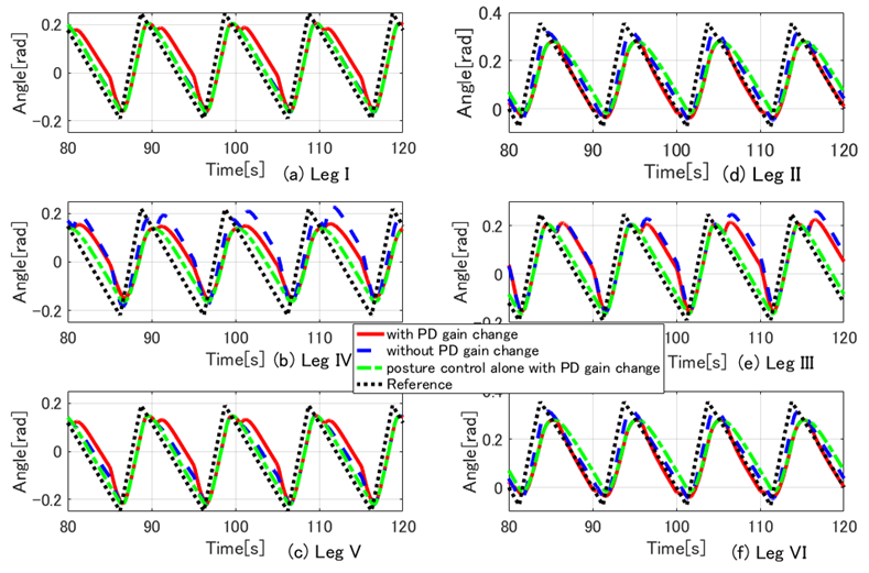
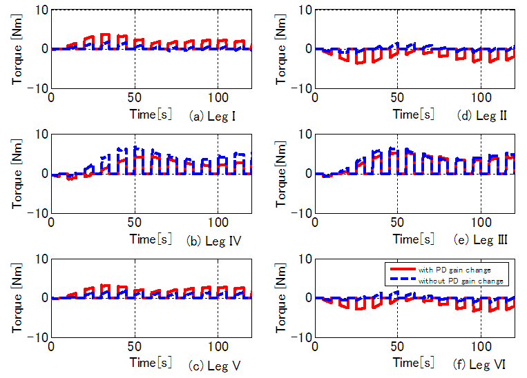
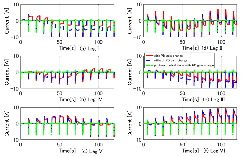
Figures 14-19 show the results of the 3D simulations, where one period is T=10 s in the three support legs, as shown in Section 3. Figures 14(a)-(f) show the time response waveform for the robot's CoG position (x, y), the yaw angle, the body height, the pitch angle, and the roll angle, respectively. Figure 15 shows the locus of the support leg position of Legs III and IV and the CoG. In Fig. 15, the locus of Leg III is on the left side and that of Leg IV is on the right side with respect to travel direction. Figure 16 shows rotating angles, Fig. 17 shows FB control inputs of the rotating link imposed by the walking directional control, Fig. 18 shows FB control inputs of the thigh link imposed by the posture control, and Fig. 19 shows FB control inputs imposed by the walking directional control. Additionally, in Figs. 16-19, panels (a)-(c) show the results for Legs I, IV, and V, while panels (d)-(f) show the results for Legs II, III, and VI. In Figs. 14-18, the blue dashed lines (Case B) indicate the results for 6-DoF control. The red solid lines (Case A) indicate the results of 6-DoF control in a situation where PD gains of the rotating links in Legs II, IV, and VI change to 0.5 times the PD gains in Legs I, III, and V. For Case A, we can consider the fluctuation of the control input to be horizontal force fluctuation. In this case, the movement range of the rotating link in Legs II, IV, and VI became 84.7% that of Legs I, III, and V. The green dash-dotted lines (Case C) indicate the results of the posture control with PD gain changes as in Case A. For case C, we do not apply the walking directional control. The black dotted line indicates the reference signal. First, we will consider Case C. In Fig. 14, where the body height and the pitch and roll angles are controlled by the posture control, posture variation is reduced. However, the body turns rightward because the tracking performance of the rotating links in the three right legs of the robot declines in comparison with that of the three left legs. In addition, since the repair motion works solely on posture control, the errors of the body position and the yaw angle can be seen to increase. Furthermore, the y-position error increases significantly because of the error of the position to land the swing leg and due to support leg slippage. The FB control inputs produced by posture control shown in Fig. 18 are generated largely at the time of support leg switching. After the support leg switching process is allowed to continue for a while, the FB control inputs decline to nearly zero. Next, we will consider Case B, in which it can be seen that the body control values follow the reference signals due to the influence of the posture and walking directional controls. Note that the tracking performance of the y-position is especially improved. This is because the FB control inputs for the rotating links (Fig. 17) in Legs III and IV work well since the reference signal of the rotating links in Fig. 16 are modified. As a result, the robot follows the target trajectory, and the error in the x-direction is reduced by the FB control input of the shank link. However, even though the body posture in terms of height, and pitch and roll angles oscillates, the body height amplitude remains within ± 0.01 m, and the pitch and roll angles are within ± 0.02 rad. Body posture oscillations become large in comparison with Case C. This is because the FB control produced by the posture control generates the control input used to eliminate the disturbance input created by the walking directional control shown in Eq. (19). This component causes the body posture oscillation. As a result, variations in the posture are small. Also, in Fig. 15, in the case of 6 DoF control, the slippage is larger in the x-direction in Leg III. In Fig. 19, the correction force acting on the shank of Leg III is larger than that on the shank of Leg IV, and the slippage of Leg III is larger than that of Leg IV due to this influence. Similar slippage occurs in the locus of other support legs. Finally, we will consider Case A, where it can be seen that the 6-DoF control shows the same trajectory tracking performance as Case B. This is because the FB control inputs of the rotating links in Legs II, IV, and VI generate negative inputs when compared with Case B, and the FB control inputs in Legs I and V generate positive inputs, as shown in Fig. 17. The three support legs on the right side move in the direction to push the body early, while the three support legs on the left side move to suppress that movement. Therefore, it can be seen that the trajectory responses of rotating links in the support phase of Legs I and V are delayed, and the trajectory responses of Legs II and VI are advanced, as shown in Fig. 16. Using these factors, the posture controller and the walking directional controller constituting the 6-DoF control generate the FB control input independently. The FB control input of the walking directional control interferes with the FB control input of the posture control, but the posture control detects the walking directional control input as a disturbance, and generates inputs to eliminate this disturbance. As a result, it can be confirmed that the proposed control method achieves 6-DoF control and that the walking directional controller is capable of generating FB control inputs that suppress effects caused by reaction force fluctuations resulting from factors such as slippage.

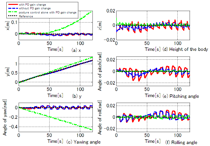Figure 14. Time responses of 6-DoF of the body in the case of walking on even terrain

Figure 15. Position of Legs III and IV in support phase

Figure 16. Time responses of rotating angles in the case of walking on even terrain

Figure 17. Time responses of FB torques for rotating links operated by the walking directional control

Figure 18. Time responses of FB inputs for thigh links operated by the posture control

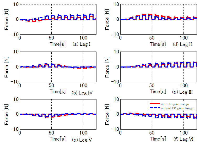Figure 19. Time responses of FB forces produced by the walking directional control

5.2. Walking on Uneven Terrain

In this section, we verify the effectiveness of our 6-DoF control method by tasking the robot with walking over irregular terrain, in this case a bump. The effectiveness of the disturbance and 6-DoF control is verified for the bump obstacle problem shown in Fig. 20. Figure 21 shows the relationship of the initial position between the bump and the robot. The bump height is 50 mm. The robot travels over the bump under the following conditions: the gait pattern is as shown in Section 3, the total walking cycle is 15 cycles, and the total walking time is 150 s. Additionally, when the robot’s CoG travels over the bump, 0.04 m is added to the reference of the body height. In this study, in order to verify the effectiveness of the control method, the reference value of the body height is automatically changed when the position of the CoG of the body is the same as that of the bump. In addition, since the reference trajectory of walking is set when the body height is zero, it is preferable to add 0.05 m to the reference signal so that the body height becomes zero. However, in order to reduce the shock at the time of walking over a bump, and to confirm the following ability to respond to a reference value fluctuation of the body height, 0.04m was added as the reference value of the body height on the bump. The contact of the swing leg with the bump was detected through the force at the leg tip and the operation of the swing leg was stopped when the force exceeded the threshold value.

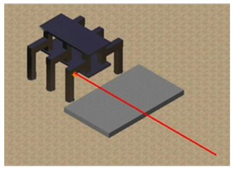Figure 20. Case of irregular terrain

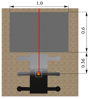Figure 21. Top view of existing step obstacle

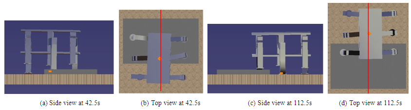
Figure 22 shows the following performance responses of the body 6-DoF, while Fig. 22 (a)–(f) show the time response waveform for the robot's CoG position , yaw angle, body height, and pitch and roll angles, respectively. In Fig. 22, the red lines indicate the results of 6-DoF control, while the blue dashed lines indicate the results of posture control alone. The black dotted lines indicate the reference signal. In Fig. 22(d), which tracks the robot’s height, the red and blue dashed lines indicate the reference signals of the 6-DoF control and posture control alone, respectively. From these figures, it can be seen that results of the body height, and pitch and roll angles in the 6-DoF control are almost the same as the results for posture control alone. This shows that the 6-DoF posture control suppresses the bump disturbance and the walking directional control FB inputs. Regarding the robot’s CoG position and yaw angle, it can be seen that the deviation from the reference signal caused by the bump and slippage only increase in cases when posture control alone is used. When 6-DoF control is utilized, the robot shows good trajectory tracking performance under walking directional control. Figures 23(a)-(d) show our animation results. Specifically, Figs. 23(a) and (b) show the side and top view at 42.5 s, respectively, while Figs. 23(c) and (d) show the side and the top view at 112.5 s, respectively. From these figures, it can be seen that the robot is controlled in accordance with the reference signals, both when climbing up and coming down from the bump. From the abovementioned results, it can be confirmed that the proposed 6-DoF control consisting of posture and walking directional control provides an effective method for a robot walking on irregular terrain.

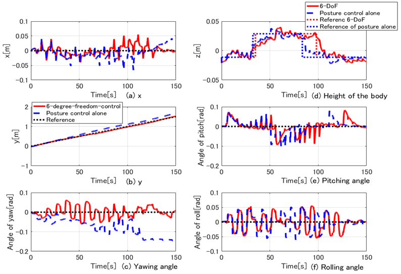Figure 22. Time responses of body 6-DoF in the case of walking on uneven terrain

Figure 23. Animation results in the case of walking on uneven terrain

6. Conclusions

In this study, a 6-DoF control method for the body of a six-legged robot was examined, and the following results were obtained:

1. As a 6-DoF control method for a six-legged robot body, a control method combining posture control, which controls the body height, and pitch and roll angles, and walking directional control, which controls the CoG position (x, y) and yaw angle, was proposed.

2. It was shown that the FB input for the thigh and shank links generated by the walking directional control interferes with the FB input for the thigh link generated by the posture control. Using 3D simulations of the six-legged robot walking behavior, it was confirmed that the FB control input produced by the posture control generated control input that eliminated the interfering control input produced by the walking directional control.

3. When varying PD gains were considered as fluctuations of the reaction force on the body caused by factors such as slippage, it was further confirmed that the results with the PD gain changes showed the almost same trajectory tracking performance as the case for no change in the gain.

4. In the case of the robot walking over a bump, it was confirmed that the proposed 6-DoF control exhibited good control performance when following the reference signals, and that the influence of the disturbance decreased.

ACKNOWLEDGEMENTS

This work was supported by JSPS KAKENHI Grant Number 25420200.