Yixiang Feng , Ichiro Kataoka
Research & Development Group, Hitachi, Ltd., Ibaraki, Japan
Correspondence to: Yixiang Feng , Research & Development Group, Hitachi, Ltd., Ibaraki, Japan.
| Email: |  |
Copyright © 2016 Scientific & Academic Publishing. All Rights Reserved.
This work is licensed under the Creative Commons Attribution International License (CC BY).
http://creativecommons.org/licenses/by/4.0/

Abstract
With the ever-growing trend of globalization, product design is often conducted collaboratively among several divisions, thus making it a huge challenge to transfer large CAE (Computer Aided Engineering) data between different locations. Our goal is to reduce the size of transfer data so that fast data transfer can be realized even when the network speed is slow. In this study, we have developed a data compression method based on TD (Tensor Decomposition). In this method, voxel simulation results data are represented as tensors and tensor decomposition based on HOOI (Higher-Order Orthogonal Iteration) algorithm is applied to the tensors. After tensor decompression, the original tensor is decomposed into a core tensor and a series of basis matrices, whose summed size is considerably smaller than that of the original tensor. As a result, a compression ratio of over 60:1 is achieved for steady flow simulation results data and the error is below 5%. A compression ratio of over 70:1 is achieved for unsteady flow simulation results data and the error is below 5%. We have confirmed that at 5% error, no significant information is lost during the data compression process. Tensor decomposition has been applied for image data compression, dimensionality reduction, and more recently for the compression of hexahedral mesh-based simulation result database. However, it is a first application of tensor decomposition to the data compression of voxel-based simulation results.
Keywords:
CAE, Product design, Signal simulation, Tensor decomposition, Data compression
Cite this paper: Yixiang Feng , Ichiro Kataoka , A Study on the Compression of Voxel Simulation Results Using Tensor Decomposition, Journal of Mechanical Engineering and Automation, Vol. 6 No. 5, 2016, pp. 95-100. doi: 10.5923/j.jmea.20160605.01.
1. Introduction
With the ever-growing trend of globalization, it is common for a company to have multiple international R&D (Research and Development) facilities that are optimized according to the company’s global business strategy. As a result, product design is often conducted collaboratively among different design sites. Collaborative global design has brought new challenges, one of which is data sharing among different sites. Most manufacturing companies use computer simulation in their product design. In product design, more accurate simulation models are required for detailed analysis. As a result, the data size became huge. For collaborative global design, it is important that the simulation database be shared within a short period of time.Methodologies for sharing data among different sites can be divided into two major categories. One is the so-called thin-client method, in which data are post-processed in servers and the generated results are transferred to client PCs as images. The other one is a direct data transfer method, in which the whole data or subsets of the data are transferred directly to the client PCs where post-processing is conducted [1]. The thin-client method is useful for easy data management and controllable information security [1]. However, the thin-client method requires real-time correspondence and therefore depends highly on the network condition and transfer speed. In the developing countries where many R&D centers are located, the network infrastructure is often poorly equipped. Based on these facts, we adopt direct transfer method in this research. To achieve the rapid processing speed required by collaborative product design, it is important to fasten the speed of data transfer. Fast data transfer can be achieved by either reducing the transferring data size, or by improving the network speed. In this research, we focus on the former approach.Data compression has long been studied in data-intensive disciplines such as image/video processing, signal processing, bioinformatics, etc. However, there were only few studies in the compression of CAE results data. In one of the studies, EZT (Embedded Zero-Tree) wavelet encoding method was used to compress BCM (Building-Cube Method)-based CFD (Computational Fluid Dynamics) results data [2]. In another study, SVD (Singular Value Decomposition) method was applied to particle simulation data [3]. Recently, high order SVD was used to compress CFD results of the outer flow around a wing with hexahedral mesh [4].TD (Tensor Decomposition), or tensor factorization, is the expansion of SVD to higher-dimensional arrays. In tensor decomposition, the original tensor is decomposed into a core tensor g and several basis matrices U V W whose total element number is equal to the dimension of the input tensor [5] [6] [7]. Figure 1 illustrates the image of tensor decomposition.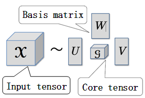 | Figure 1. Image of Tensor Decomposition |
Tensor decomposition has been applied for image data compression [8], dimensionality reduction [9], and more recently for the compression of hexahedral mesh-based simulation result database [4]. However, to the best of our knowledge, there has been no application of tensor decomposition to the data compression of voxel-based simulation results. In this study, we propose a data compression method for voxel simulation results based on tensor decomposition.
2. Tensor Decomposition
2.1. Theory of Tensor Decomposition
Tensor decomposition can be formulated as an optimization problem of minimizing the distance between an input tensor and its approximate tensor of a lower rank. Mathematically, it is written as Eq. (1): 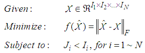 | (1) |
where  is the Nth-order input tensor consisting of real numbers. Ii is the dimension of the ith-mode and Ji is the rank of the ith-mode.Two popular tensor decomposition schemes are CP decomposition, where the core tensor is diagonal [10], and Tucker decomposition, where the core tensor is dense [11] [12]. In this research, we use Tucker decomposition due to its flexibility in controlling the approximated tensor through adjusting the size of the core tensor. In Tucker decomposition, the approximated tensor
  is decomposed as shown in Eq. (2):
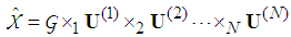 | (2) |
where  is the core tensor and
 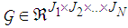 .
.  is the basis matrix and
 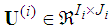 .In this research, we adopt the HOOI (Higher-Order Orthogonal Iteration) tensor decomposition algorithm proposed by Lathauwer et al. [13] [14]. Using HOOI, the core tensor
  can be calculated using the following equation.
 | (3) |
The basis matrix  is calculated using an ALS (Alternating Least Squares) method which is an expansion of the Least Squares method. The initial basis matrices are calculated using the HOSVD algorithm [13]. That is to say,
  is calculated as the left singular vector of the ith mode expansion of
  .
.
2.2. Tensor Decomposition as a Data Compression Method
One important property of tensor decomposition is that the overall size of the core tensor and basis matrices is usually much smaller than that of the original tensor. We take advantage of this property and use tensor decomposition for lossy data compression.CR (Compression Ratio) is defined as the number of elements before and after tensor decomposition.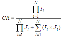 | (4) |
The approximation error caused by tensor decomposition is defined as follows.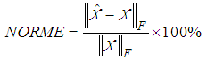 | (5) |
where NORME is the approximation error based on the Frobenius norm. The Frobenius norm is defined as follows. | (6) |
where xi is the elements of the tensor  .
.
3. Test Results
3.1. Test Model
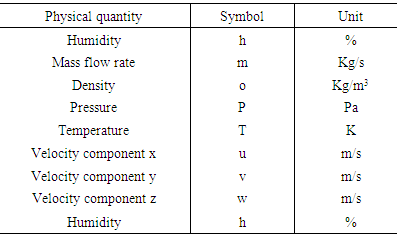
In this study, we use voxel–based simulation to generate simulation results. Voxel simulation is sometimes used to simulate thermal fluid phenomena for actual industrial products due to the simplicity and robustness of grid generation [15] [16] [17]. In voxel simulations, the simulation models tend to be huge because of the fact that the voxel grids have to be divided at a high resolution to ensure precision [15]. Therefore, it is even more important to compress the voxel-based simulation results when transferring the database.Figure 2 shows the voxel simulation model used for testing. In voxel simulation, the 3D simulation volume is automatically divided into orthogonal grids and then thermal or fluid simulations are performed. Our model is a simplified inverter model, which consists of fan unit, bus bar, resistors, etc. Thermal and fluid simulations are performed in the 3D volume containing these parts. The fan unit is regarded as fluid since it is the duct for air flow. The number of cross sections along the Z-axis is 251 and the number of voxels in the X and Y axes are 156 and 125, respectively. Therefore, the total number of voxels in the test model is 251x156x125=4,894,500. We performed simulation of air flow using in-house voxel simulation software and obtained results for eight physical quantities. Table 1 shows a list of physical quantities of the test model.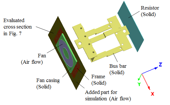 | Figure 2. Test model |
Table 1. List of physical quantities of the test model
 |
| |
|
To test data compression of 4th–dimensional simulation data, we also perform unsteady flow simulation for 10 time steps.All calculations are performed on an HP Z800 PC with CPU of Intel Xeon W5590 @ 3.33 GHz and 32GB physical memory.
3.2. Evaluation of Compression Ratio
First, we represent simulation results of one time step with a 3rd-order tensor and then perform tensor decomposition. The three dimensions of the 3rd-order tensor correspond to the X, Y and Z axes of the voxel model. For comparison, we also expand the input simulation results data to 2D matrix and perform SVD. Figure 3 shows a comparison between TD and SVD in terms of compression ratio and approximation error. The X-axis is compression ratio and log scale is used. It is obvious that, at any error level, TD has higher compression ratios than those of SVD. For example, when approximation error is 5%, the compression ratio for SVD is about 5.4, while for TD it is about 60.0 and is about 11 times over that of SVD.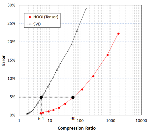 | Figure 3. Comparison between TD and SVD (3rd-order) |
Next, we represent the 10-step time series of voxel simulation results with a 4th-order tensor and then perform tensor decomposition to compress the data. The four dimensions of the 4th-order tensor correspond to the X, Y, Z axes and t (time) of the voxel model. Figure 4 shows a comparison between TD and SVD in terms of compression ratio and approximation error. The X-axis is compression ratio and log scale is used. Similar with the results of the 3rd-order tensor, when error level is the same, TD gains higher compression ratios than SVD does. For example, when error is 5%, the compression ratio for SVD is about 4.0, while for TD it is about 70.0, which is about 17 times over that of the SVD. Comparing with the results of 3rd-order tensor, the compression ratio for 4th-order tensor is higher than that of the 3rd-order tensor, which suggests that TD is suitable for the compression of large-scale and high-dimensional database.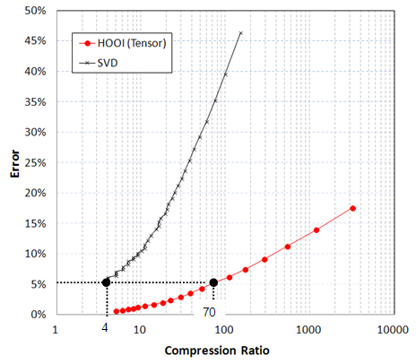 | Figure 4. Comparison between TD and SVD (4th-order) |
3.3. Computational Time
Figure 5 shows the comparison of computational time between TD and SVD in terms of compression ratio.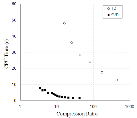 | Figure 5. Comparison of CPU time in terms of CR |
As shown in Figure 5, the computational time of TD is about an order greater than that of SVD, which is due to the complexity of the HOOI algorithm. The HOOI algorithm requires SVD to be calculated in each mode and iterates until the ALS algorithm converges [14].It is also observed from Figure 5 that TD and SVD operate at different zones. TD is more time-consuming, but the compression ratio is much higher than that of the SVD. However, it is not sufficient to look at the compression ratio alone, because there is a tradeoff between the compression ratio and approximation error.Figure 6 shows a comparison of computational time between TD and SVD in terms of approximation error. 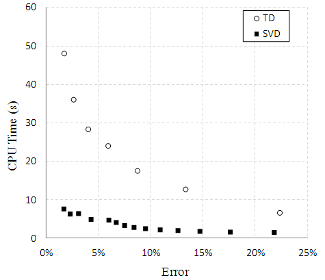 | Figure 6. Test result of hierarchical tensor decomposition |
It is observed from Figure 6 that the computational time for TD is considerably greater than that for SVD. When the approximation error is 5%, the computational time for TD is about 25s, while for SVD it is about 5s. It should be noted that when the compression error is the same, the compression ratio of TD is much greater than that of SVD, as shown in Figure 3 and Figure 4. We conclude that there is a tradeoff between the performance and computational time. To reduce the calculation time of TD is one of our most important future tasks.
4. Results and Discussion
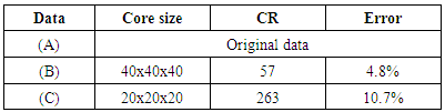
To further investigate the information loss caused by data compression, we compare the data before and after compression by visualizing the data. Figure 7 shows the pressure distributions in the cross section of the air flow inside the fan unit. The core sizes, compression ratio and error are listed in Table 2. It can be seen from Figure 7 and Table 2 that, with the increase in core tensor size, the pressure distribution in the cross section gradually approximates that of the original data. When the approximation error is 10.7%, the overall feature of the pressure distribution is captured, but there are still noticeable differences in the color tone and some other details. Meanwhile, when the approximation error is decreased to 4.8%, there is no noticeable difference between the compressed data and the original data, which suggests that the compressed data can be used for further analysis or design.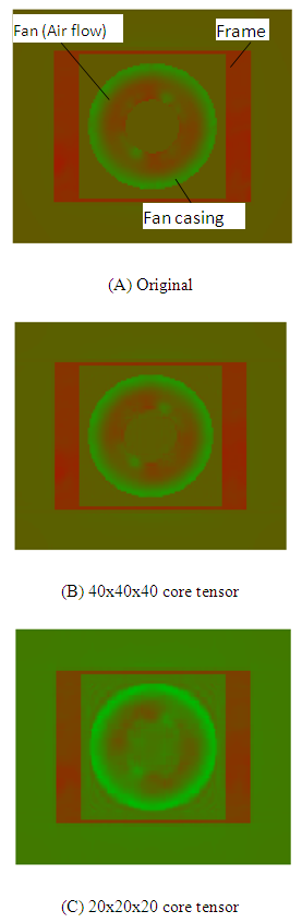 | Figure 7. Navigation data demodulated by tracking loop |
Table 2. List of physical quantities of the test model
 |
| |
|
We also compare the data before and after data compression of the unsteady flow simulation results. Figure 8 shows pressure distributions in the cross section of the air flow inside the fan unit, which is the same cross section as used in Figure 7. In Figure 8, the nth row corresponds to the simulation results of the nth time step, where n is a number between one and ten. The first column is the original data without data compression. The second column is the data after data compression with TD at a compression ratio of 3174. The third column is the data after data compression with TD at a compression ratio of 52. The fourth column is the data after data compression with SVD at a compression ratio of 10. It can be observed from Figure 8 that, at compression ratio 52, the compressed data from TD yields almost the same pressure distributions as those from the original data. Meanwhile, for the compressed data from SVD, even at compression ratio 10, there are considerable differences between the compressed data and the original data. Even though the overall pressure distributions look similar, the data compressed from SVD lose many of the detailed characteristics in the pressure distribution. Therefore, it is confirmed that data compression using TD outperforms data compression using SVD.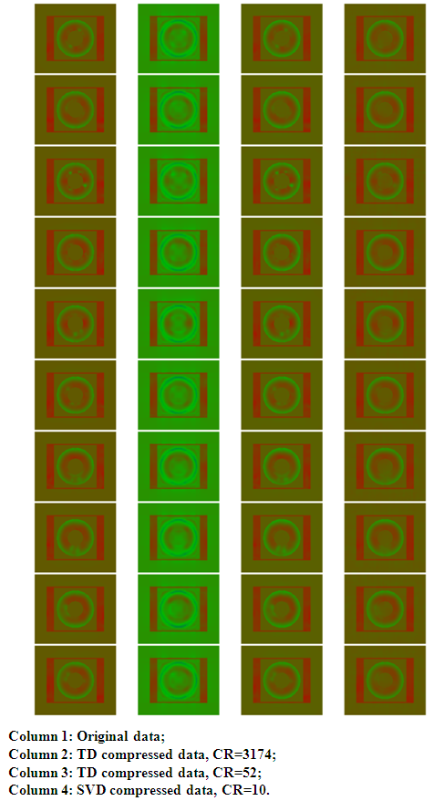 | Figure 8. Comparison of data compression results for unsteady flow simulation results data |
5. Conclusions
We proposed a data compression method for simulation results database using tensor decomposition. We verified the method in a simplified inverter model and obtained the following conclusions.(1) We represent single voxel simulation results data with 3rd-order tensor and decompose it. As a result, we obtain a compression ratio of 1:60 while the approximation error is about 5%. Compared with traditional method in which the compression ratio is about 5.4, the compression ratio of our method is more than 10 times higher.(2) We represent a time-series of voxel simulation results data with 4th-order tensor and decompose it. As a result, we obtain a compression ratio of 1:70 while the approximation error is 5%. The proposed method is over 17 times higher in terms of compression ratio as compared with traditional method in which the value is about 1:4.(3) Computation time for TD is greater than that for SVD. There is a tradeoff between performance and computational time.
References
| [1] | D. Matsuoka, F. Araki, Survey on Scientific Data Visualization for Large-scale Simulations, JAMSTEC Report of Research and Development, Vol. 13, (2011) 35-63. (in Japanese). |
| [2] | R. Sakai, D. Sasaki, S. Obayashi K. Nakahashi, Wavelet-based data compression for flow simulation on block-structured Cartesian mesh, International Journal for Numerical Methods in Fluids, Vol. 73, Issue 5, (2013) 462–476. |
| [3] | K. Wada, K. Iwasaki, Compression of Particle-based Fluid Simulation Data, Information Processing Society of Japan, Kansai Branch, (2011). (in Japanese). |
| [4] | L.S. Lorente, J.M. Vega, A. Velazquez, Compression of aerodynamic databases using high-order singular value decomposition, Aerospace Science and Technology, Vol. 14, No. 3, (2010) 168-177. |
| [5] | T.G. Kolda, B.W. Blder, Tensor decomposition and applications, SIAM Review, Vol. 51, No. 3, (2009) 455-500. |
| [6] | E. Acar E., B. Yener, Unsupervised multiway data analysis: a literature survey, IEEE Transactions on knowledge and data engineering, Vol. 21, No. 1, (2009) 6-20. |
| [7] | L. Qi, W. Sun, Y. Wang, Numerical multilinear algebra and its applications, Front. Math. China, Vol. 2, No. 4, (2007) 501-526. |
| [8] | D. Vlasic, M. Brand, H. Pfister, J. Popovic, Face transfer with multilinear models, ACM Trans. Graphics, Vol. 24 (2005) 426-433. |
| [9] | H. Wang, N. Ahuja, A tensor approximation approach to dimensionality reduction, Intl. J. Comput. Vis., Vol. 76, (2008) 217-229. |
| [10] | R.A. Harshman, Foundations of the PARAFAC procedure: Models and conditions for an explanatory multi-modal factor analysis, UCLA Working Papers in Phonetics, Vol. 16 (1970) 1-84. |
| [11] | L.R. Tucker, The extension of factor analysis to three-dimensional matrices, in Contributions to Mathematical Psychology, H. Gulliksen and N. Frederiksen, eds., Holt, Rinehart & Winston, New York, (1964) 109-127. |
| [12] | L.R. Tucker, Some Mathematical Notes on Three-Mode Factor Analysis. Psychometrika, Vol.31, No.3, (1966) 279-311. |
| [13] | L.D. Lathauwer, B.D. Moor, J. Vanderwalle, A multilinear singular value decomposition, SIAM J. Matrix Anal. Appl., Vol. 21, No. 4, (2000) 1253-1278. |
| [14] | L.D. Lathauwer, B.D. Moor, J. Vanderwalle, On the best rank-1 and rank-(R1,R2,..., RN) approximation of higher-order tensors, SIAM J. Matrix Anal. Appl., Vol. 21, No. 4, (2000) 1324-1342. |
| [15] | T. Tawara, K. Ono, Fast large scale voxelization using a pedigree, the 10th ISGG Conference on Numerical Grid Generation, Sep. 16-20, Forth, Crete, Greece, (2007). |
| [16] | M. Ikegawa, H. Mukai, M. Watanabe, Airflow-simulation by voxel mesh method for complete hard disk drive structure, IEEE Trans. Magn., Vol. 45, No. 11, (2009) 4918-4922. |
| [17] | S. Hayashi, M. Watanabe, Y. Iwase, K. Kanno, K. Fujimori, Development of a household vacuum cleaner with a new cyclone dust collector, FEDSM2007-37014, (2007) 1925-1932. |

 Abstract
 Reference
 Full-Text PDF
 Full-text HTML