R. Nagai, Y. Tabata, M. Sadatomi, A. Kawahara, A. Santoso
Department of Advanced Mechanical Systems, Graduate School of Science and Technology, Kumamoto University, Japan
Correspondence to: R. Nagai, Department of Advanced Mechanical Systems, Graduate School of Science and Technology, Kumamoto University, Japan.
| Email: |  |
Copyright © 2016 Scientific & Academic Publishing. All Rights Reserved.
This work is licensed under the Creative Commons Attribution International License (CC BY).
http://creativecommons.org/licenses/by/4.0/

Abstract
The present study is concerned with the pressure loss due to 60 degree Y-branch in horizontal mini-channel with a rectangular cross-section of 2.5 mm height × 4.6 mm width in the upstream channel and of 2.5 mm height × 2.36 mm width in the downstream channels. The pressure loss, the gas phase velocity and the void fraction in the channels upstream and downstream from the branch were measured, and analysed. Since no correlations of the respective parameters has found, the new correlations has been proposed and their validity against the present experimental data has been clarified.
Keywords:
Rectangular mini-channel, Two-phase flow, Y-branch, Pressure drop
Cite this paper: R. Nagai, Y. Tabata, M. Sadatomi, A. Kawahara, A. Santoso, Experimental Study on Two-Phase Pressure Drop through Horizontal Mini-Channel with Y-Branch, Journal of Mechanical Engineering and Automation, Vol. 6 No. 4, 2016, pp. 78-84. doi: 10.5923/j.jmea.20160604.02.
1. Background
Gas-liquid two-phase flow in mini-channels is a phenomenon seen in compact chemical reactors and heat exchangers with phase change, e.g., air conditioners and cooling devices. These devices contain flow channels of various cross-sections, e.g., circular and rectangular, as well as various types of singularities, e.g., branches, sudden expansions, sudden contractions, bend, and so on. In particular, there are many configurations of the branches, i.e., the impacting T-junction and the side branches with various angles. In order to design and develop the mini-size heat exchanger with the side branches, a full understanding of the characteristics of two-phase flow through the branch and the pressure gradient in the channels upward and downward from the branch in various flow regimes is essential.Ito and Imai (1973) measured the single-phase pressure drop in equal-sided impacting T-junctions of circular cross-section of 35 mm I.D. with various curvature radii and geometrical shapes of joining edge. The experiments were conducted at two inlet Reynolds numbers of Re = 1 × 10⁵ and 2 × 10⁵. They reported a correlation for the pressure loss coefficient as a function of the split ratio and the curvature radius and the joining edge. Oka and Ito (2005) studied tees and wyes with the large area ratios of the inlet channel to the outlet channel. For the tees, the test section had an inlet channel of 54.03 mm I.D. and outlet ones of two different sizes of 54.03 mm and 15.97 mm. All experiments were conducted with a fixed inlet Reynolds number of Re = 1 × 10⁵. A correlation was proposed for the pressure loss coefficient through the tee as a function of the split ratio and the inlet to outlet area ratio. Elazhary and Soliman (2012) studied the single- and two-phase pressure drops in a horizontal mini-channel with an impacting T-junction with a rectangular cross-section of 1.87 mm height × 20 mm width. The correlations for the single-phase and two-phase pressure losses were proposed relating to the inlet flow rates of gas and liquid, the split ratio. All these studies are concerned with impacting T-junctions and there are a few on the studies on the two-phase flows through Y-branch, and nothing on mini-channels with the Y-branch.The first objective of the present study is to obtain experimental data on the pressure distribution along the test channel with 60 degree Y-branch with a rectangular cross-section, the gas phase velocity and the void fraction in the channels upstream and downstream from the branch. The channel is mini sized one placed on a horizontal plane and has dimensions of 2.5 mm height × 4.6 mm width in the upstream channel and of 2.5 mm height × 2.36 mm width in the downstream channel. The second one is to analyse the data with models and correlations relating to the data to determine their accuracy in prediction. The third one is to propose the respective new correlations. A result of such experiment, analysis and proposal is described in the present paper.
2. Experimental Method
2.1. Experimental Apparatus
Figure 1 shows a top view of the present mini test channel with Y-branch placed on a horizontal plane. The test channel has a rectangular cross-section, and is made of transparent acrylic resin for visual observation.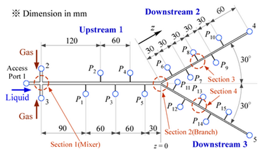 | Figure 1. Top view of mini test channel with Y-branch |
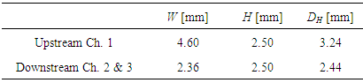
Table 1 shows the cross-sectional dimensions of the channel cross-section: the width (W), height (H) and the hydraulic diameter (DH). They are 4.60 mm, 2.50 mm and 3.24 mm for the upstream Ch.1, while 2.36 mm, 2.50 mm and 2.44 mm for the downstream Ch. 2 and Ch. 3, thus the ratio of contraction σA is approximately 0.52. Among 20 connecting taps, the tap #1 is the liquid phase inlet port while the taps #2 and #3 are the gas phase inlet ports. Therefore, the gas-liquid two-phase flow starts from section 1. The taps #4 and #5 are the outlet ports of the flow. P1 to P15 are the pressure taps, and the pressure at P4 was measured with a gauge type pressure transducer (FP101-L31-L20, Yokogawa). The pressure at other pressure tap was determined from the pressure difference measured with a differential pressure transducer (DP15-32 and DP15-26 depending on the pressure range) between the tap and P4 tap. The accuracy of the pressure measurement was confirmed within 3.5 Pa from a calibration test.Table 1. Channel width, height and hydraulic diameter, respectively for Ch. 1 to 3
 |
| |
|
Figure 2 shows the present apparatus. Water as the test liquid was introduced from a tank to the test channel by a pneumatic-type pump via a flow control valve and a liquid flowmeter. The pump consisted of a pressure vessel containing water and pressurized air from a compressor for pushing the water surface in the vessel. This pump gave a steady pulsation-free liquid flow. Air as the test gas was introduced from a compressor to the test channel via a pressure regulator, a flow control valve, and a gas flow meter.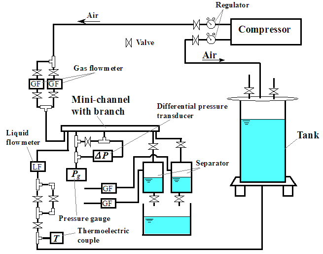 | Figure 2. Experimental apparatus |
The liquid and the gas flow rates introduced were read from calibrated mass flow meters (FD-S and FD-A1, both KEYENCE Co., Ltd.). In order to obtain accurate time averaged values of air and water flow rates and pressures, the output signals from the respective sensors were fed to a personal computer via A/D converter at nominally 1 kHz over 10 sec. The liquid flown from the outlet of Ch. 2 and 3 were separated from air in the respective separators, and their flow rates were measured by weighting the liquid discharged over a sufficient period of time using a small container and an electric balance (200±0.001 g, SHIMADZU Co). The liquid split ratio from Ch. 1 to Ch. 3, RL = QL3/QL1, was controlled with a flow control valve between the outlet of Ch. 2 and the separator for Ch. 2, by taking care of the water levels in the separators of Ch. 2 and 3 to remain the same height. The airs separated in the respective separators were lead to the respective dry-type gas volumetric flow meters. In order to confirm the accuracy of the respective outflows, the authors checked the total mass flow rate of Ch. 2 and 3 to agree with the mass flow rate of Ch. 1, respectively for water and air. If the agreement was worse than 10 % to the flow rate of Ch. 1, the data was discarded.The flows in three observation area of section #3 (Ch. 1), section #4 (Ch. 2) and section #5 (Ch. 3) in Fig. 1 were observed with a high-speed video camera (VH-Z00R, KEYENCE Co., Ltd.) in order to determine the respective flow patterns. Besides the above measurements, the gas phase velocity, uG, in two-phase flow was measured with the high-speed video camera, and the void fraction, α, was determined by substituting the measured uG and the superficial gas velocity, jG (= QG / (W⋅H)), into α = jG/uG.
2.2. Experimental Conditions
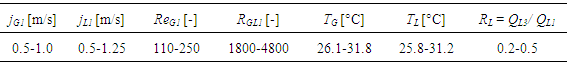
The ranges of the liquid and the gas superficial velocities, jL,1, jG,1 at z = -30 mm, a point 30 mm upstream from the Y-branch and the liquid split ratio, RL, in the present experiments are listed in Table 2. The superficial velocity is the volume flow rate divided by cross-sectional area of flow channel. Since the static pressure dropped gradually from the channel inlet to outlet, the superficial velocity of gas, jG, increased along the channel axis. Thus, jG, at z = -30 mm in Ch. 1, z = 30 mm in Ch. 2 and Ch. 3 were used in the discussion of gas phase velocity and void fraction data. Flow regimes covered are all slug flows in Ch. 1 but include a little bubble flow in Ch. 2 and 3.Table 2. Flow and temperature conditions of the present experiments
 |
| |
|
3. Results and discussion
3.1. Gas Phase Velocity and Void Fraction
The gas phase velocity, uG, data for all channels were plotted against the total superficial velocity, j (= jG + jL) as shown in Fig. 3. The solid and broken lines represent the calculations by the following homogeneous flow model, Eq. (1), and drift flux model by Zuber and Findlay (1965), Eq. (2), with Mishima and Hibiki’s C0 correlation (1996), Eq. (3): | (1) |
 | (2) |
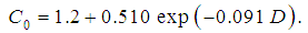 | (3) |
Here, the drift velocity, VGj, was taken as zero since the flow is horizontal. Eq. (3) was based on air-water two-phase flow data in vertical circular pipes of 1 to 5 mm I.D., where D is the inner diameter of the pipe in mm. In the present study, D was replaced by the hydraulic diameter, DH, because of rectangular channel.The uG data distribute a little higher than the line of homogeneous flow model (uG = j), but do not agree with uG = 1.63 j. Thus, the distribution parameter, C0, was modified as follows: | (4) |
Fig. 4 shows that the calculated uG by Eqs. (2) and (4) agree with the present data within 12% in average for all channels.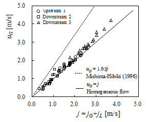 | Figure 3. Gas phase velocity data for Ch.1, Ch.2 and 3 against total superficial velocity |
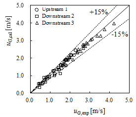 | Figure 4. Comparison of gas phase velocity between experiment and calculation by drift flux model with Eq. (4) for the distribution parameter |
The void fraction, α, data was obtained by substituting uG data into α = jG/uG. These data are compared with the following three correlations: (a) homogeneous flow model (α = β), (b) Armand’s correlation (1946), α = 0.833β, and (c) the present correlation using Eqs. (2) and (4). Where β(= jG/j) is the gas volume flow fraction. Figs. 5 (a) – (c) show the assessment results of the three void fraction correlations. In a low void fraction range, the data agree well with the calculation by the homogeneous flow model. While in a high void fraction range, the data agree well with the calculation by the present correlation.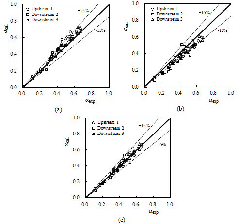 | Figure 5. Comparison of void fraction between experiment and calculations by three correlations (a) Homogeneous low model, (b) Armand’s correlation, (c) The Present correlation |
The prediction errors by each correlation are 7.5%, -10.4%, and 0.1% for the average relative error, εM, and 12.7%, 13.5% and 9.5% for the root mean square relative error, εRMS.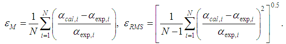 | (5) |
Here, N is the number of the data points. The minimum errors for the whole data were obtained by the present correlation.
3.2. Axial Pressure Distribution and Branch Pressure Drop
Figure 6 shows typical results on the axial pressure distributions measured for a slug flow at jG1 = 0.75 m/s and jL1 = 1.0 m/s, and at the split ratio of liquid of RL = 0.8. The gradient of two-phase frictional pressure drop in Ch. 1, Ch. 2 and 3, (dpf /dz)1, (dpf /dz)2 and (dpf /dz)3, is obtained by fitting the pressure distribution data in each channel with the least-square method. The pressure changes across the Y-branch, Δp2 and Δp3, the pressure changes between Ch. 1 and 2 and Ch.1 and 3, are determined by the extrapolations of the respective pressure distributions. In the present paper, Δp3 is used as the representative because the Δp2 is relatively small and tend to have a poor accuracy. 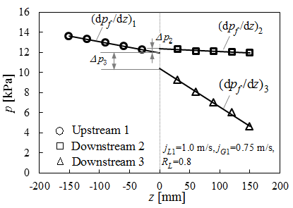 | Figure 6. Pressure distribution along the channel axis |
The pressure change,  , is the sum of the reversible and the irreversible changes,
  and
and 
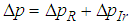 | (6) |
 | (7) |
Here, ρL and ρG are the liquid and air densities. In the present study, the terms relating air dynamic pressure in Eq. (7) are neglected because air density, ρG, is much smaller than the liquid density, ρL. The experimental data on the irreversible change, ΔpIr, was determined from Δp data by subtracting calculated ΔpR.Figures 7 (a) - (c) show the ΔpIr3 data for the branch from Ch.1 to Ch. 3 at three liquid split ratio of RL = 0.8, 0.7 and 0.6. The abscissa is the volumetric quality at Ch. 3. The symbols in each figure are labelled depending on liquid superficial velocity in Ch. 1, jL1. ΔpIr3 increases with increasing of jL1 at a fixed RL and β3. In addition, at a fixed jL1, ΔpIr3 is roughly constant and independent of β3.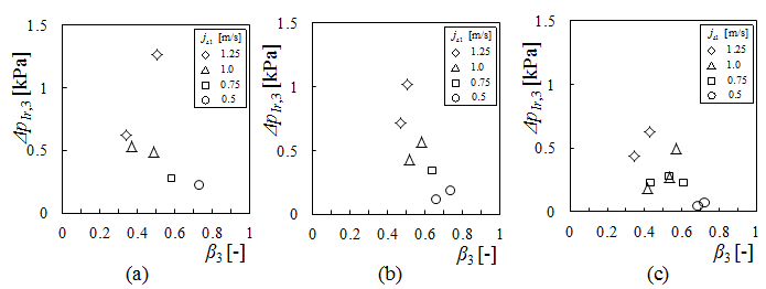 | Figure 7. Irreversible pressure change at branch versus volumetric quality (a) RL = 0.8, b) RL = 0.7, (c) RL = 0.6 |
In the present study, the branch pressure loss-coefficient, kb, is defined as: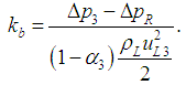 | (8) |
The branch loss-coefficient data is plotted against the volumetric quality in Ch. 3 in Figs. 8 (a) - (c) for each RL. Although ΔpIr3 data depend on jL1 as the mentioned above, but kb data do not dependent so much on jL1 and are roughly constant of kb = 0.30.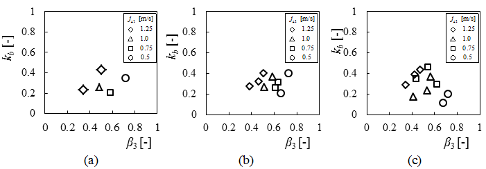 | Figure 8. Pressure loss-coefficient against gas volumetric flow ratio (a) RL = 0.8, (b) RL = 0.7, (c) RL = 0.6 |
3.3. Prediction of Irreversible Pressure Loss at Branch
If the inlet and the outlet gas and liquid superficial velocities and liquid physical properties are given, the irreversible pressure loss due to the branch, ΔpIr, can be predicted from Eq. (9), being the same as Eq. (8), with kb = 0.3 together with Eqs. (2) and (4) for uG calculation.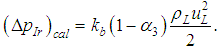 | (9) |
In order to validate the present prediction method on the two-phase irreversible pressure loss due to the branch, the calculation value, (ΔpIr)cal was compared with the present data, (ΔpIr)exp. The average error and the root mean square error of ((ΔpIr)cal - (ΔpIr)exp / (ΔpIr)exp) are 17.2% and 45.4%. Figure 9 shows the comparison between the experiment and the calculation. In the case of jL1 = 0.5 m/s, the average of relative error is 45.7% and root mean square of that is 88.9%, while in the case of other jL1, the average of relative error is 8.6% and root mean square of that is 28.5%. Therefore, it can be concluded that the present method can predict the irreversible pressure loss due to the branch within r.m.s. error of 28.5% if jL1 ≥ 0.75 m/s.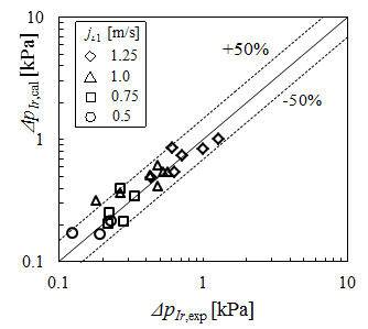 | Figure 9. Comparison of irreversible pressure loss between the present calculation and the present experimental data |
4. Conclusions
Air-water two-phase flow experiment was conducted at room temperature and atmospheric pressure using a horizontal rectangular mini-channel with a Y-branch. The width and height were from 4.6 mm by 2.5 mm to 2.36 mm by 2.5 mm. From the analyses of the experimental data, the followings can be clarified:1. The gas phase velocity data did not fit well the calculations by the homogeneous flow model and the drift flux model with Mishima and Hibiki’s C0 correlation. However, by modifying C0 correlation, the calculation by the drift flux model agreed well with the present experiment data.2. The void fraction prediction based on the above gas phase velocity calculation method agreed well with the experimental data within r.m.s error of 9.5 %.3. The irreversible pressure loss-coefficient due to branch, kb, was roughly constant of 0.30, independent of jL1, β3 and RL.4. The present calculation on the irreversible pressure loss due to the branch agreed with the present experimental data within r.m.s. error of 28.5% if jL1 ≥ 0.75 m/s.
ACKNOWLEDGEMENTS
The present study was partially supported by KAKENHI (26420118).
References
| [1] | Ito, H., Imai, K. (1973). Energy losses at 90° pipe junctions. ASCE J. Hydraulics Div.99, 1353 – 1368. |
| [2] | Oka, K., Ito, H. (2005). Energy losses at tees with large area ratios. J. Fluids Eng. 127, 110 – 116. |
| [3] | Elazhary, A. M., Soliman, H.M. (2012). Single- and two-phase pressure losses in a horizontal mini-size impacting tee junction with a rectangular cross-section. Experimental Thermal and Fluid Science 41, 67-76. |
| [4] | Zuber, N., Staub, & Findlay, J. A. (1965). Average Volumetric Concentration in Two Phase Flow Systems. Trans, ASME, J. Heat Transfer, 87, 453 -468. |
| [5] | Mishima, K., & Hibiki, T. (1996). Some Characteristics of Air-water Two-phase Flow in Small Diameter Vertical Tubes. Int. J. Multiphase Flow, 22 – 4, 703 – 712. |
| [6] | Armand, A. A. (1946). Resistance to Two-phase Flow in Horizontal Tube (in Russian). Izv.VTI, 15, 16 - 23. |

 Abstract
 Reference
 Full-Text PDF
 Full-text HTML