Daniel Hutzschenreuter1, Frank Härtig1, Klaus Wendt1, Ulrich Lunze2, Harald Löwe3
1Physikalisch-Technischer Bundesanstalt, Braunschweig, Germany
2University of Applied Science Zwickau, Zwickau, Germany
3Technische Universität Braunschweig, Braunschweig, Germany
Correspondence to: Frank Härtig, Physikalisch-Technischer Bundesanstalt, Braunschweig, Germany.
| Email: |  |
Copyright © 2015 Scientific & Academic Publishing. All Rights Reserved.
This work is licensed under the Creative Commons Attribution International License (CC BY).
http://creativecommons.org/licenses/by/4.0/

Abstract
In various areas of industrial manufacturing the correct evaluation of Chebyshev geometrical elements has fundamental importance for inspection of products with Coordinate Measuring Machines (CMM). According to standard ISO 1101 these are the default algorithms for accessing form deviation and to calculate certain datums for the evaluation of position deviation. To validate the accuracy of these computations, a network of National Metrological Institutes (NMIs) and Designated Institutes (DIs) established an online service which, among other tests, allows manufacturers and users of CMM software to test their mathematical algorithms for Chebyshev. The test covers five important types of associated geometrical elements which are calculated by the so-called Minimum-Zone criterion (MZ). By registration at the TraCIM (traceability for computationally-intensive metrology) online service a user can order the test for validation of his algorithms. Each test contains fifty individual data sets. The users’ evaluation results are compared against reference results provided by the institution offering the test. Procedures for the comparison cover numerical uncertainties of the reference results and maximum permissible errors (MPEs) specified by the user. For each test an online report including detailed test results is issued. Test data, test procedure and test evaluation are subjected to quality rules specified and controlled by TraCIM e.V. which is an international head organization for metrological algorithm validation.
Keywords:
Chebyshev, Minimum-Zone, TraCIM, Software Validation, Geometrical Elements, Coordinate Metrology
Cite this paper: Daniel Hutzschenreuter, Frank Härtig, Klaus Wendt, Ulrich Lunze, Harald Löwe, Online Validation of Chebyshev Geometric Element Algorithms Using the TraCIM-System, Journal of Mechanical Engineering and Automation, Vol. 5 No. 3, 2015, pp. 94-111. doi: 10.5923/j.jmea.20150503.02.
1. Introduction
3D Coordinate Metrology is an essential part of different industrial sectors such as automotive, mechanical and medical engineering in order to meet the steady growing demands on quality of products. A key requirement of 3D Coordinate Measuring Machine (CMM) software is therefore the correct fitting of ideal geometrical elements for point data that is extracted from the surface of features from work pieces. The underlying computational aims are mathematical approximation problems. In general solving these problems requires the application of different numerical algorithms. Conventional calibration of CMM principally utilizes reference artefacts like block gauges, calibration cubes or spheres or complex artefacts like ball plates. Their associated measurands are connected with the meter definition by a chain of precedent calibration. Obviously calibration with artefacts uses only a small amount of algorithms that are available at CMM. Hence calibration results give limited conclusion on the overall accuracy and stability of the software used. Therefore, autonomous testing of software components with test data is a convenient and cost-efficient supplement for conventional calibration.ISO 10360 series [1] and VDI 2617 [2] specify requirements for the calibration of CMM. A wide area of independent software testing remains unhandled by these standards. Only in ISO 10360 part 6 basic procedures for testing least squares (Gaussian) geometrical element algorithms are described. Actual there is no test available according to that standard. A similar development is the least squares element test from [3]. The NMI of Germany – PTB (Physikalisch-Technische Bundesanstalt) has been offering this test to industry for more than 20 years. Other important fitting algorithms are Minimum-Zone best-fit (Chebyshev), Maximum-Inscribed and Minimum-Circumscribed geometrical elements. The calculation of these elements needs the application of considerably more complex numerical algorithms than those which are used for least squares evaluation. However, regulations on software tests for Chebyshev elements are least developed in standardization. Urgently needed tests have not been available for industrial applications until now.To overcome this critical situation PTB in cooperation with the University of Applied Science in Zwickau has established a test for Chebyshev geometrical element algorithms according to the Minimum-Zone best-fit criterion. The test is referred to as Chebyshev test and comprises the evaluation of five important geometrical elements. These are line and circle in 2D space as well as plane, sphere and cylinder in 3D space. In total one test comprises fifty individual data sets. The test is implemented within the scope of a software validation online service that was established in 2014 during an European research project named Traceability for computationally-intensive metrology (TraCIM) [4]. It offers a web interface including a web shop [5] and a client-server application for testing of metrological software. It is available from any location worldwide with an internet connection. This service is referred to as TraCIM service. Figure 1 depicts the general concept.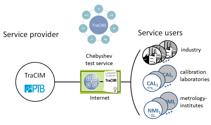 | Figure 1. TraCIM Service for Validation of Chebyshev Algorithms |
A NMI, which in this case is PTB, provides the test service. This is of paramount importance, since the tests are to be carried out – or at least monitored – by the supreme metrological authority of a country. PTB is organized with other metrology institutes under the umbrella of the TraCIM association (TraCIM e. V.). It’s main task consists in describing unified quality rules and in defining the technical infrastructure under which the algorithm tests are to be run. Each provider is, however, sole responsible and also held liable for the correctness and reliability of the tests. The NMIs act autonomously in defining the test scope, the business workflow, in the maintenance of their datasets, the running of the server and in consultation and support for customers. For this reason, each metrology institute runs its own TraCIM web shop and server. Each server has to be addressed individually, which leads to a different extent of services offered depending on each metrology institute. The metrology institutes, however, have the possibility of providing algorithm tests mutually as subcontractors, which allows a test provider to enhance the extent of services offered.The primary users of the TraCIM service are manufacturers of analysis and evaluation software for measuring instruments. The service allows them to have their analysis algorithms validated and officially approved by an national metrology institute. This mainly serves to increase confidence in the products they offer on the market. In principle, they can have this service unlocked for their customers in order to have, for example, updates validated directly on the user’s computer. Software engineers can already test their algorithms during the development phase to be on the safe side and, thus, make development faster. New customers who want to access the service need to register once and can access individual tests via the internet afterwards. The service is available 24 hours a day at each day of the year at each location on the globe.The following sections give details on the implementation of the Chebyshev test within the TraCIM system. After an introduction to the mathematical computation for the geometric elements of interest the TraCIM test design and requirements for an successful implementation of the test are presented. It comprises specific technical requirements and business aspects associated with testing. A marginal part provides details on the general TraCIM System that apply to all existing and future tests. These are the TraCIM quality rules, IT architecture and the basic test procedure which are provided for completeness of the explanations but are not the core issue of the paper. Further sections will give important details on the creation of the test data and the assessment of associated numerical uncertainties for Chebyshev geometric elements. Finally five public test data sets with reference results are presented.
2. Mathematical Background
Clear specification of computational aims for the calculation of Chebyshev geometrical elements is fundamental for a traceable validation of algorithms. This requires a unambiguous definition of input data, appropriate output parameters and the mathematical model which links the input with the output for correct calculation. Figure 2 outlines these properties for fitting a 2D circle with the MZ criterion.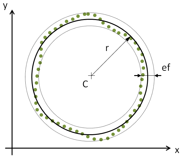 | Figure 2. Outline of a 2D circle associated with a point cloud by MZ Criterion |
The input data is a finite set of point coordinates which represent the extracted contour of a real circular feature. In the sequel this set is called a point cloud. The output parameters give a 2D circle with ideal geometrical shape and a quantity for the form deviation. The parameters of the circle are the center point  and the radius
  . The form deviation is two times the maximum orthogonal distance between all points of the point cloud and the circle. It is denoted by
  . Under assumption of the MZ criterion the objective is to find output parameter values with the smallest possible form deviation. In Fig. 2 this property is depicted by two concentric circles that are adjacent to the point cloud. The area between both circles contains all points and has minimum width. The associated Chebyshev circle is the median circle of the adjacent elements.In accordance to the previous example general definitions for Chebyshev computational aims are made in the sequel. After giving detailed specifications for each geometrical element of interest the section is concluded with remarks on approaches for calculation of the Chebyshev elements.
2.1. Chebyshev Computational Aims
For  the point cloud is a set of Cartesian coordinates
  with
with  for all indices
  in index set
  . In case of 2D elements
  there is
  . Else for 3D elements
  there is
  .Further let
  denote a vector that gives the output parameters of the associated geometrical element. The amount of parameters depends on the individual element and values are restricted to a specific permissible range
  .The orthogonal distance between points
  and the lateral surface of the geometrical element with parameters
  is calculated by the distance function
 . The terms
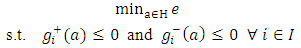
  are frequently used in further descriptions.Then the computational aim for calculation of Chebyshev geometrical elements with the MZ criterion is to solve
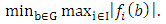 | (P) |
 parameter vector
 permissible parameter value range
 index of point
 index set of point cloud
 orthogonal distance functionIn (P) the term
 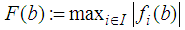 is minimized. This meets the requirement of geometrical element fitting with the smallest possible form deviation which computes as
  . Individual definitions of parameters and distance functions for the geometrical elements 2D line, 2D circle, plane, sphere and cylinder are listed below. Note, the chosen parameterization agrees with recommendations from ISO 10360 part 6. Moreover the definition of some parameters depends on the centroid
  of the point cloud. It is defined by equation (1).
 | (1) |
 centroid of point cloud
 amount of points in point cloud
 location vector of point
2.1.1. Specification for 2D Line
The geometrical element is defined by two parameters. The first are Cartesian coordinates  of a point on the line. For a unique definition this point may be calculated as the projected centroid that is the point on the line with shortest distance to the point cloud centroid. The second parameter is the orientation vector
  giving the direction of the line. Its length is constraint to
  . In total there are four different parameter values. These are assigned to the parameter vector
  with value range
 . Term
  denotes the unit sphere in ℝ2. Moreover
  is a constraint for the definition of the projected centroid. Equation (2) gives the orthogonal distance function for 2D line.
 | (2) |
 index of point
 parameter vector
 location vector of point
 projected centroid on 2D line
 vector orthogonal to 2D lineVector
  is orthogonal to
  . Note, that the scalar product used for 2D line is the Euclidian product
  in ℝ2.The solution of (P) for the 2D line may be depicted by a pair of parallel lines. All points of the point cloud are enclosed between these lines. The orthogonal distance of the lines is the smallest possible to enclose all points. Then the Chebyshev 2D line is the median line of the pair of lines with minimum distance. The form deviation is the orthogonal distance of the outer adjacent lines.
2.1.2. Specification for 2D Circle
The parameters of the associated 2D circle are the center point  and the radius
  . There are no additional constraints on the parameter definition. The parameter vector is
  . Its permissible value range is
  ℝ2×ℝ+. Equation (3) gives the orthogonal distance function for the 2D circle.
 | (3) |
 index of point
 parameter vector
 location vector of point
 center point of 2D circle
 radius of 2D circleFor an arbitrary
 ℝ2 the norm calculates as
  . These definitions and (P) conclude the basic description of the Chebyshev 2D circle from Figure 2.
2.1.3. Specification for Plane
Geometrical element plane has two parameters. Its position is defined by the Cartesian coordinates  of a point on the plane. For a unique definition of the plane it may be calculated as the projected centroid that is the point on the plane with shortest distance to the point cloud centroid. The second parameter is the orientation vector
  . It gives the normal of the plane. The length of the vector is constrained to
  . In total there are six different parameter values defining the plane. These are assigned to the parameter vector
  . Valid values
  are within the parameter range
 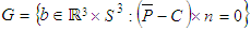 . Term
  denotes the unit sphere in ℝ3. Moreover
  is a constraint for the definition of the projected centroid. The operator × in the previous term is the cross product in ℝ3. It is defined by
 The orthogonal distance between the plane and the points from the point cloud is calculated by (4).
 | (4) |
 index of point
 parameter vector
 location vector of point
 projected centroid on plane
 normal vector of planeNote, that the scalar product used for the plane is the Euclidian product
  in ℝ3.The solution of (P) for the plane could be depicted by a pair of parallel planes. All points of the point cloud are enclosed between these planes. The orthogonal distance of the planes is the smallest possible to enclose all points. Then the Chebyshev plane is the median plane of this pair of planes. The form deviation is the orthogonal distance of the outer adjacent planes.
2.1.4. Specification for Sphere
The parameters of the associated sphere are the center point  and the radius
  . There are no additional constraints on the parameter definition. The parameter vector is
  . Its permissible value range is
  . Equation (5) gives the orthogonal distance function for the sphere.
 | (5) |
 index of point
 parameter vector
 location vector of point
 center point of sphere
 radius of sphereFor an arbitrary
  ℝ3 the norm calculates as
  .The solution of (P) for the sphere may be depicted by a pair of concentric spheres. All points of the point cloud are enclosed between the lateral surface of both spheres. The radius difference between the spheres is the smallest possible distance to enclose all points. Then the Chebyshev sphere is the median sphere between the pair of concentric spheres. Further the form deviation is the difference of radii between the outer adjacent spheres with minimum distance.
2.1.5. Specification for Cylinder
The geometrical element for cylinder is defined by three parameters. The first parameter gives the position of the cylinder axis. It is denoted by  and may be calculated as the point on the cylinder axis with shortest distance to the point cloud centroid (projected centroid). The second parameter gives the orientation vector
  of the cylinder axis. It is constraint to
  . Finally the third parameter is the radius
  In total there are seven different parameter values assigned to the parameter vector
  . The parameter range is
 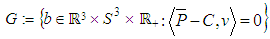 . Condition
  implies that
  is the projected centoid.Equation (6) gives the orthogonal distance function between the lateral surface of the cylinder and points from the point cloud.
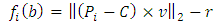 | (6) |
 index of point
 parameter vector
 location vector of point
 projected centroid on cylinder axis
 direction vector of cylinder axis
 radius of cylinderThe norm is the same as defined in (5). Further the cross product in ℝ3 is used for calculation of the distance between
  and the cylinder axis.The solution of (P) for the cylinder can be depicted by a pair of coaxial cylinders. All points of the point cloud are enclosed between the lateral surface of both cylinders. The radius difference between the cylinders is the smallest possible distance to enclose all points. Then the Chebyshev cylinder is the median cylinder between the pair of concentric cylinders. Further the form deviation is the difference of radii between the outer adjacent cylinders with minimum distance.
2.2. Outline of Chebyshev Element Calculation
Problem (P) is a non linear minimax program (MP) in mathematical optimization theory [6], [7]. The difficulty for a direct solution with an appropriate numerical algorithm for MP is the insufficient smooth objective. E. g. the terms  are not continuous differentiable in
  . Hence other approaches need to be applied. Frequently this requires the transformation of (P) into an ordinary non linear constraint program. Let
  denote a new parameter that is an upper bound for
  . Then
  is equivalent to
  and
and  for all
  . The parameter vector is extended to
  with the new permissible value range
  . Further there is
 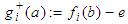 and
and 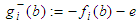 for all
  . With these preliminary definitions the transformed computational aim for Chebyshev elements is given by (P’).

 (P’)
(P’) extended parameter vector
 permissible value range of
 half form deviation value
 index of point
 index set of point cloud
 constraint function of point
 constraint function of point
  General methods for solving problems of type (P’) are presented in [8]. These are for example penalty-barrier-methods or sequential-quadratic-programs. More specific calculation methods applicable for the MZ criterion with distance functions (2) – (6) are presented in [9], [10], [11], [12] and [13].Finally the existence and uniqueness of a solution for (P) and likewise (P’) majorly depends on the structure of the point cloud. Basic recommendations for feasible input data are listed below.• For element 2D line the point cloud should at least have three pairwise different points.• For element 2D circle the point cloud should at least have four pairwise different points that are not collinear.• For element plane the point cloud should at least have four pairwise different points that are not collinear.• For element sphere the point cloud should at least have five pairwise different points that are not coplanar.• For element cylinder the point cloud should at least have six pairwise different points that are not coplanar.Moreover, in the case of symmetric point clouds there may exist multiple equivalent solutions for the Chebyshev computational aim (P).
3. TraCIM Quality Rules
The correctness of the results, the liability of the service as well as the unambiguous rules and descriptions for using of test procedure are essential demands which guarantee an unproblematic and user-friendly service. Therefore, the TraCIM e. V. specified quality rules which have to be followed by all institutes offering the TraCIM test. Below the most important are listed:§1. Each institute providing tests is liable for the correctness of the reference results.§2. Input values and its associated uncertainty values are defined as error free.§3. Reference parameters and their associated uncertainty must be provided.§4. The test data have to be verified successfully by at least three independent software applications.§5. Tests shall provide only one unambiguous result.§6. Test cases shall reflect common practical situations.§7. Clear description of the tests procedure, parameters to be calculated and validation criterion have to be provided.§8. It is recommended to provide public test data and reference parameter.§9. All data sets sent and received as well as all test reports are subject to archiving.In opposite to an academic view all of the quality rules are targeting pragmatic handling of software tests.
4. IT-Architecture of TraCIM System
PTB provides the TraCIM service by running a server with the TraCIM system application for software testing. It is a worldwide accessible, long-term usable and easy to maintain online application for testing metrological algorithms. TraCIMs’ IT architecture consists of four central modules (Figure 3). The web shop is the user interface [5]. Similar to online shopping, interested service users have to get registered via the Internet before they are able to order individual tests. Internally, the web shop is directly connected with the server core application for automated processing of incoming requests such as orders, requests for test data and evaluation of calculated test results.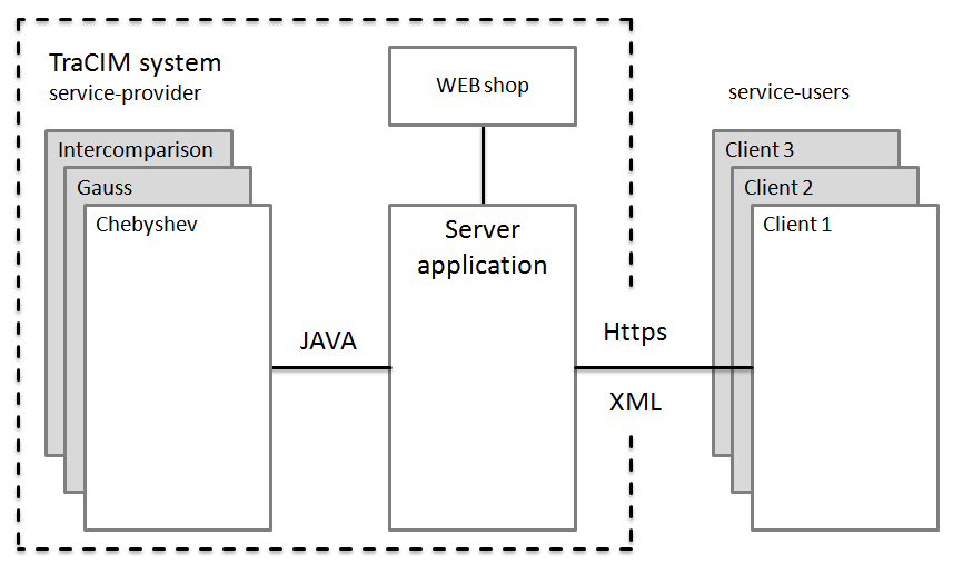 | Figure 3. Modular IT-Architecture of TraCIM System |
The core application is a management module, which is operated by a competent metrology institute. It manages all of the operating data and controls the data flow to the other modules.The expert modules are developed by experts and provide individual tests. Each expert module operates basically autonomously and deals with all logical operations in connection with a test. It makes the test data sets available on request, compares the results computed by the service user (customer) with its own reference results and, finally, issues the test report. Since the individual tests may vary significantly from one application to the other, only few input parameters have been defined by TraCIM for the data traffic between the expert modules and the core application. This applies, for instance, to the support of a software interface in JAVA which allows the expert system to be logged into the server system. Basic processing of data such as unique keys identifying each test and each request are transmitted via this interface. The formatting of the test data may be freely selected, the expert is, to a large extent, free to generate the test data according to his needs. Therefore, new tests and special data structures such as for implementing test cases for Chebyshev geometrical element software can easily be integrated into the TraCIM system.The formal specification of the TraCIM client-server interface is more restrictive in contrast. The communication runs via a REST interface that is a special type of Https connection. Hereby, the data are being embedded into an XML structure. Then again, within this structure, free formats of test data (such as binary formats or established test data structures) can be defined, depending on the application. The expert module is solely responsible for defining the test data format, generating the test data and analysing the calculated results.
5. Test Design and Processing Data
Figure 4 shows the detailed flow chart for the test of Chebyshev algorithms starting from user registration at the web shop site until issuing the test report.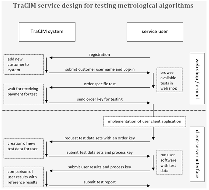 | Figure 4. Flowchart for performing an software test offered by the TraCIM System |
5.1. Registration
In order to get access to the TraCIM service any customer must at first register at TraCIM system. PTB’s TraCIM web shop (http://tracim.ptb.de) provides a fully automated online registration form. A service user must provide valid contact information like company name, address, phone number and e-mail address. It is essential for PTB to have this information in order to carry out any business activities associated with issuing official test reports and to provide appropriate support. After registration the account data including a unique customer ID, user name and password are generated automatically by the TraCIM system and submitted to the service user by e-mail. These are necessary for further communication with the server and for ordering tests. Registration is free of any charge for all service users.
5.2. Order of PTBs’ Chebyshev Test
A valid TraCIM account allows the service users to order individual tests for validating their software. Login at the TraCIM web shop site gives access to a test ordering area. Here the service user may select the test for Chebyshev algorithms. There are two different offers. One is the test with public data at no charge. It should be used preferably to verify the correct implementation of the client-server communication before ordering test data subject to charge. The service user may order this test at any time. The test can be repeated an unlimited number of times. No fees are claimed. The second offer is directed at customers who want to receive an official test report signed by PTB. This test must bepurchased. Therefore, TraCIM office sends a payment request to the service user by e-mail. After payment is received the validation test will be enabled and an order key is automatically generated and send to the service user by e-mail. The order key allows the service user to identify all tests he ordered in the customer area of the web shop.
5.3. Implementation of a Test Client
The technical requirement for performing a TraCIM test is that a service user provides a client application for requesting test data from and submitting calculated results to PTB’s TraCIM server. For communication with the TraCIM server a client application must use an Https (Hypertext Transfer Protocol Secure = encrypted Https) connection that allows to send and receive content in the form of character strings, which in case of Chebyshev algorithm tests are messages in XML format. Each Https connection is generated from a specific URL (Uniform Resource Locator), i.e. for requests of test data or requests of the test result. After opening the connection according to URL the following configurations must be done:• Enable output and input operations for the connection.• Set the request method “GET” in case of test data request.• Set the request method “POST” in case of test result transmission.• Set connection property “content-Type” to “application/xml”.• Set connection property “accept” to “application/xml”.• Set connection property “content-length” to the amount of characters of the content that is send to the TraCIM system.Service users are advised to use the free-of-charge public test data for checking the correct communication between their client application and the TraCIM server before performing validation tests subjected to charge. Software packages for creation and configuration of Https connections are available for different programming languages such as for example• Java: java.net API (HttpURLConnection)• C/C++: Microsoft C++ REST SDK (“Casablanca”) or similar• C#: System.Net (.NET 4.5: System.Net.Http ) Assembly
5.4. Requesting Test Data Sets
For test data requests the service user has to contact the TraCIM server using the client application. The necessary Https connection must be configured for a ‘GET’ request and is opened with the following predefined URL that contains the order key.https://tracim.ptb.de/tracim/api/order/<ORDER_KEY>/testAfter receiving the request the server application verifies the order key. If the order key is valid the server returns a message containing the test data in a special XML format. A detailed description of the data structure is given in the section on Chebyshev test data. Test data sets are not send by the server, if the test has already been send to the service user, if the identification is unknown or if the validity of the test has expired.For each test data set the TraCIM system generates a corresponding ‘process key’ in order to clearly identify the data set. It also allows to assign messages transmitted via the internet connection to individual test data and to a particular testing process. The process key is submitted together with the test data sets to the service user.
5.5. Send Calculation Results for Evaluation
The service user evaluates the test data sets and calculates parameter values of the associates Chebyshev geometrical elements by his software. For validation the results have to be written in a predefined XML structured message which is in detail described in the upcoming section on user results.The service user should submit the message with his results to TraCIM server with the client application. The necessary Https connection must be configured for a ‘POST’ request and is opened with the following predefined URL.https://www.tracim.ptb.de/tracim/api/test/<PROCESS_KEY>The address must contain the process key which the service user has received together with the test data sets.
5.6. Receiving the Test Report
After receiving results of the software under test the TraCIM system verifies the validity of the process key. If the key is accepted, the correctness of the results is tested and a report on the outcome is created. It states, whether the application software of the user has computed correct results for the underlying test data sets or not. The report is send back to the service users’ client application within a XML message whose content is schematically shown below.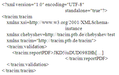 The element ‘tracim:reportPDF’ contains the test report, which is a ‘base64’ encoded character string. The service user has to decode it into an easy readable pdf-file.User results are not accepted by the server if they were already send, if the process key is unknown or if the validity of the test has expired.
5.7. Costs
The validation of mathematical software algorithms is subject to charges. This has several reasons: firstly, the service user receives an official report on the evaluation, secondly, the management and maintenance of the TraCIM system generates costs, and, last but not least, the development costs for the system need to be refunded in the long run. Figure 5 shows the prices for testing of Chebyshev algorithms.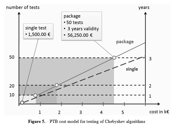 | Figure 5. PTB cost model for testing of Chebyshev algorithms |
There are different offers. Besides a single test, also test packages of 10, 20 and 50 tests will be available.Purchasing test packages makes sense, for example, in case of a software-developing company willing to have its updates or upgrades validated regularly.The test is provided by PTB since March 2015. Strictly speaking, a validation is valid only for the software used in the test. Only the software manufacturer can appraise when a modification in his complex analysis software could have impact on the result of the computation. It is therefore his responsibility vis-à-vis his customers to assess whether the validation is still valid or whether the validation must be repeated.
5.8. Availability of the Service
Order keys for single tests and test packages have time-limited validity for testing which is shown in Figure 6. A single test may only be performed once. For additional tests a service user must purchase new order keys. In opposite order keys for packages are applicable multiple times according to the amount of tests within the package. If all tests are consumed the order key is not valid anymore.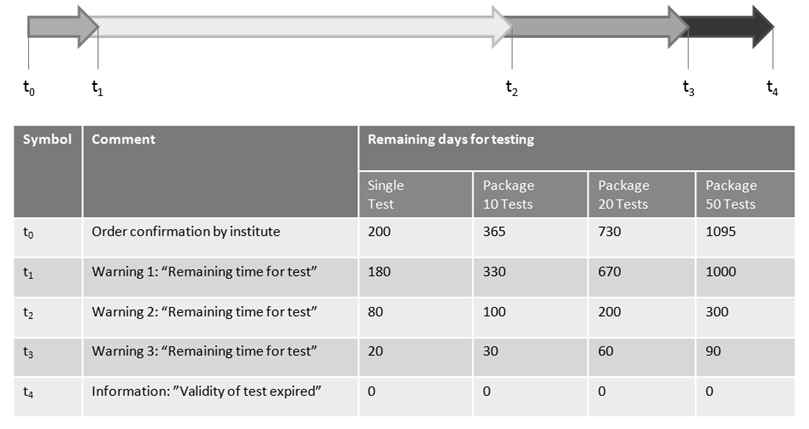 | Figure 6. Outline on regular TraCIM system information on remaining days for using TraCIM service before expiration of order key |
The TraCIM system regularly informs a service user on the remaining time for performing tests by e-mail. An initial message is sent when a service user gets the order key at day  . Interim messages follow giving information on the remaining time for testing and in case of test packages the remaining number of available test runs. If the service user does not test his software by the expiration date a final message is send that the order key will lose its validity at day
  .
.
5.9. Test Data
5.9.1. General XML Data Structure
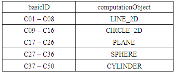
Test data denotes the input values for algorithms to be tested, which are automatically transmitted by the TraCIM system to the service user. For PTB’s Chebyshev test this comprises 50 different points clouds. The number of points per data set varies between 10 and 631. Figure 7 shows the general XML data structure of the test data.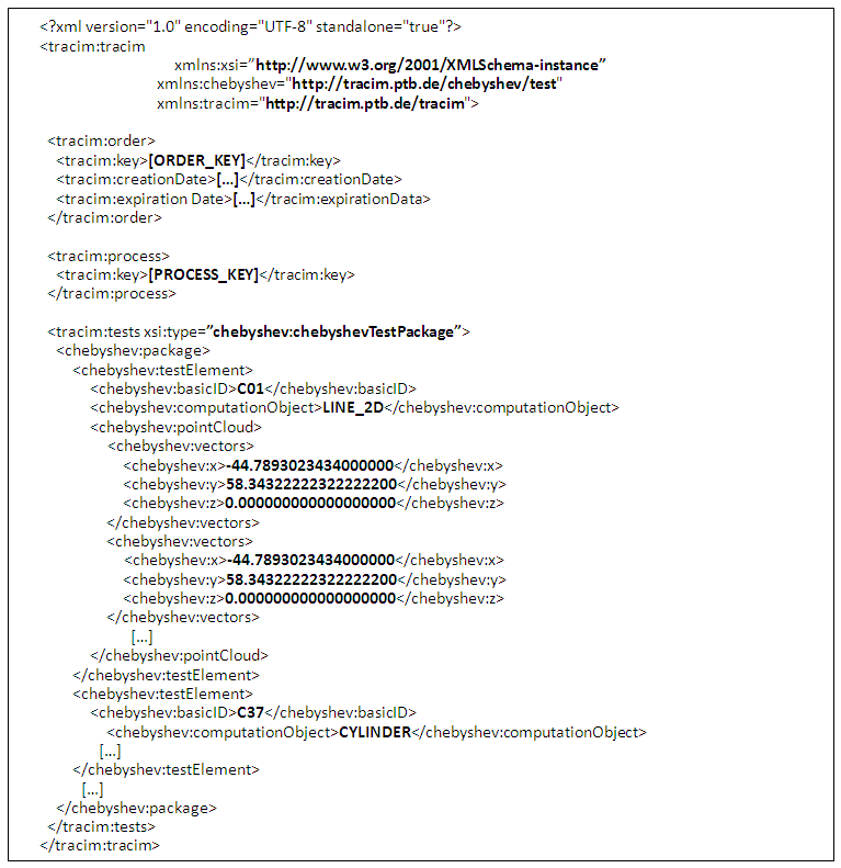 | Figure 7. General XML Data Structure for Test Data |
The test data that is returned by the TraCIM system is composed according to an XML scheme with three major elements for order identification, process identification and the test data sets. The order element contains a copy of the order key, a date of the creation of the test data and a date for the expiration of the test data (deadline for sending test results for evaluation).The process element contains the process key associated with the test data request. The test element is of type ‘chebyshevTestPackage’.It contains a list with fifty different ‘testElement’ entries. Each of these elements gives a unique data set ID (‘basicID’), the point cloud and the geometrical element that must be fitted to the point cloud (‘computationObject’). Table 1 provides a list of all entries for the data set ID element and the computation object element.Table 1. Data Set IDs and Associated Geometric Elements
 |
| |
|
There are eight data sets for testing Chebyshev 2D line, eight data sets for Chebyshev 2D circle, ten data sets for Chebyshev plane, ten data sets for Chebyshev sphere and fourteen data sets for Chebyshev cylinder. The points of a point cloud are given by ‘vector’ elements. Each vector gives the  and
and  coordinate values of one point. Properties of the values are• Each point coordinate value is delivered as decimal number with 20 digits and scientific e-format. The values refer to the unit mm (millimeter).• All point coordinates are within the value range [-500 mm, +500 mm].• For LINE_2D and CIRCLE_2D the z-component of each point is set zero (x, y, 0) as these are 2D elements.Note, that the restriction to the unit mm and value range is subject to future change. Newer versions of the TraCIM test may accept customer defined unit and range.The test data sets are stored within a database that is connected with PTB’s expert module for testing Chebyshev algorithms. Whenever a service user requests test data fifty sets of test data are randomly selected from that data base and send to the service user.
5.9.2. Test Data Design
Point clouds for Chebyshev algorithm testing were created with a generator software which was developed at University of Applied Science Zwickau (https://www.fh-zwickau.de). The tests cover data sets with points that are both randomly and systematically distributed on fragments of the geometrical elements mainly representing full features with different random and systematic form deviation components. A few datasets represent partial features. The data sets are designed to have only one unique solution when calculating the associated geometrical element with the MZ criterion according to formula (P). The functionality of the data generator for the Chebyshev test is shown in Figure 8.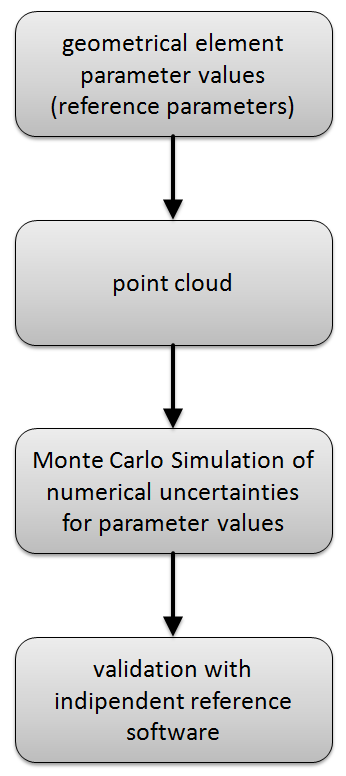 | Figure 8. Outline of Chebyshev Test Data generation procedure |
Input for the test data creation are values for geometrical parameters of the Chebyshev elements. In the first step the generator software calculates a point cloud from these input parameters. Basic algorithmically approaches for the creation are presented in [14] and [15].The point data set has the property that the preset parameter values give a sufficiently accurate reference solution for the fitting problem (P) with the generated point cloud. Hence the input parameters are used as reference parameters for PTBs’ Chebyshev algorithm test. The second step of the generator procedure evaluates numerical uncertainties of the reference parameter values. Here an Monte Carlo Simulation method is applied. It evaluates the change in parameter values for the solution of (P) due to small perturbation within the input point cloud. Thereby a random noise with relative magnitude  is added to each coordinate value of all points in a data set. Later the reference parameters and their associated uncertainties are used at the test evaluation. Finally the last step of the generator software is a validation of parameter values and point clouds. The accuracy of the reference result is simply checked by comparison with parameter values calculated by a reference software for the Chebyshev element fitting.
5.10. User Results
For submitting computation results, which have been obtained by use of the software under test, to the TraCIM system the data structure in Figure 9 applies.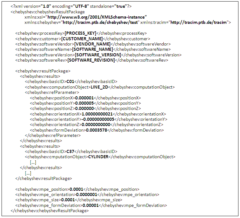 | Figure 9. General XML Data Structure for submitting User Results |
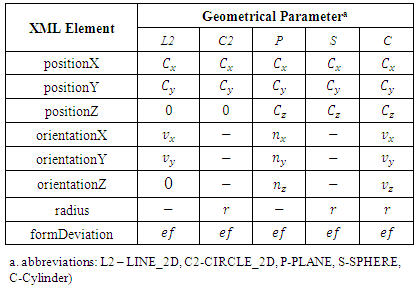
The root element of the XML structured content is the ‘chebyshev Result Package’. It contains information on the software under test, a ‘resultPackage’ element with the geometry parameter values calculated by this software and MPE (maximum permissible error) values for the test of the accuracy of the software results. A user has to give the following information on the test process and tested software:• [PROCESS_KEY]: the key that was send with the test data (Fig. 7)• [CUSTOMER_NAME]: user name from TraCIM system registration• [VENDOR_NAME]: name of the software vendor• [SOFTWARE_NAME]: name of software that computed the test results• [SOFTWARE_VERSION]: version of software that computed the test results • [SOFTWARE_REVISION] revision of software that computed the test resultsThe ‘resultPackage’ element must contain a list of fifty ‘results’ elements. For each point cloud of the test data there has to be one ‘result’. The different elements are identified by the basic IDs and computational objects according to Table 1. The parameter values of the tested software are written to the ‘refParameter’ element. Table 2 shows which parameter values a user has to write into the XML structure for each geometrical element belonging to the test.Table 2. Specification of User Result Parameters
 |
| |
|
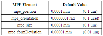
The geometrical element parameters are those from section 2. In case of 2D elements line and circle the z-component of the position parameter has to be zero. Moreover the user must write zero for the z-component of the orientation in case of the 2D line. For 2D circle and sphere the orientation elements must not be defined in the XML data structure. Similar the radius element must not be written for 2D line and plane.Further the values provided by the user have to fulfil the following requirements:• All parameter values must be in decimal number format with the maximum amount of decimal digits the tested software provides (fixed point or floating point e-format are applicable).• Only a dot is allowed as separator of decimal places for all values. • The usage of a comma is forbidden within any decimal value.• The values for position, radius and form deviation refer to the unit mm (millimeter).• Radius and form deviation must be positive values. Finally the client has to specify the MPE values for position, orientation, size and form deviation that should be used for test evaluation. User MPE values are subjected to unit millimetre for length and rad for orientation. The default values for PTBs‘ Chebyshev test are presented in Table 3. User specified values for the MPEs must be greater or equal to the default values. Details on the application of the MPE values at test evaluation are presented in the following section.Table 3. Default MPE Values for Chebyshev Test
 |
| |
|
All values that are entered into the schema must meet the previous specifications. The XML schemata for the Chebyshev test is downloadable from the following URLs:Test data schema:https://tracim.ptb.de/tracim/api/schema/PTBWHZ_MATH_CHEBYSHEV_v1_test.xsd;User result schema:https://tracim.ptb.de/tracim/api/schema/PTBWHZ_MATH_CHEBYSHEV_v1_result.xsd;Report schema:https://tracim.ptb.de/tracim/api/schema/tracim.xsd.Service users are advised to utilize these schemata during client development in order to check a proper functioning with the client.
5.11. Test Evaluation
Accessing the accuracy of software is carried out by comparison of calculated user parameter values with the reference results of PTB for each geometrical element. Thereby deviations between user results and reference results are computed by four different types of test parameters. These are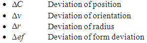 The calculation of
  is individual for each geometrical element. In the case of 2D line the position deviation is the orthogonal distance between the line position of the user and the reference line. For circle and sphere it is the distance of user center point and reference center point. For element plane the test parameter computes as the orthogonal distance of the user plane position and the reference plane. Finally at evaluation of cylinder results the position deviation is the orthogonal distance between the user position of the cylinder axis and the reference cylinder axis.The test parameter for the orientation deviation is applied for elements 2D line, plane and cylinder. It calculates the sine of the angle between user orientation vector and reference orientation vector. The orientation vectors are the direction vector of 2D line and cylinder axis as well as the normal vector for element plane.For elements 2D circle, sphere and cylinder the radius deviation is the amount of the difference between user radius value and reference radius value.For all elements
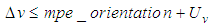
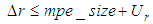
  is the amount of the difference between user form deviation value and reference form deviation value.For test evaluation these test parameters are compared with the user specified MPE bounds for maximum permissible deviations. The evaluation takes the numerical uncertainties of the reference parameter values into account. Equations (7)-(8) show the principal test criteria.
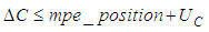 | (7) |
 | (8) |
 | (9) |
 | (10) |
 numerical uncertainties
 is the numerical uncertainty for the position deviation
  due to the uncertainty of the reference position parameter value.
  is the numerical uncertainty for the orientation deviation
  due to the uncertainty of the reference orientation parameter value.
  is the numerical uncertainty of the reference radius value and
  is the numerical uncertainty of the reference form deviation value. All uncertainty values are separately calculated for each of the 50 tested elements by a Monte Carlo simulation with the test data and reference results. The values represent extended measurement uncertainties with covering factor
  [16].A customer passes the Chebyshev algorithm test if for each of the fifty test data sets conditions (7)-(10) hold.If for any user result one of the previous defined conditions is not satisfied then the test report will give a table with individual evaluation results for each test parameter and each test data set.
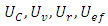
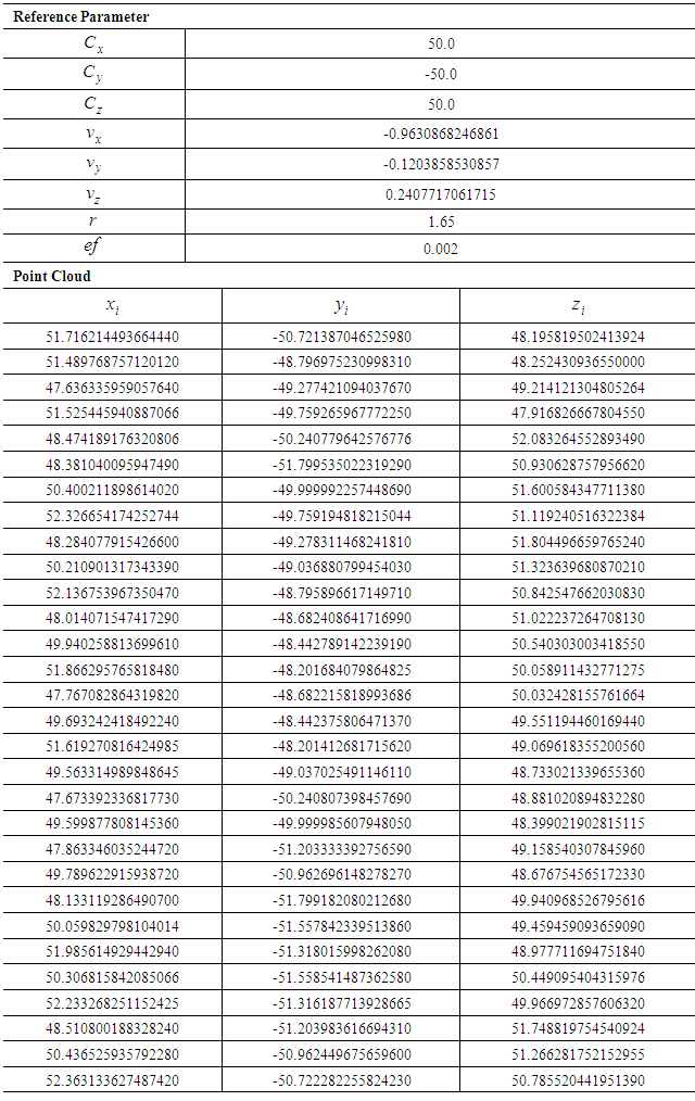
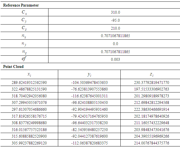
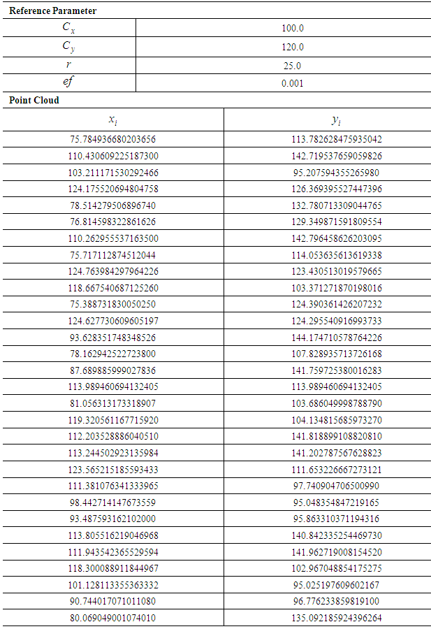
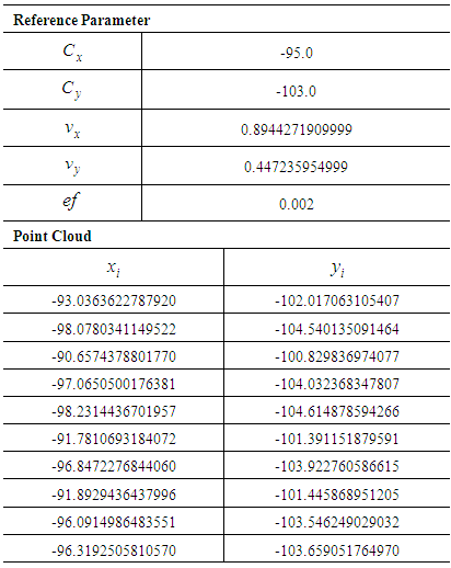
6. Public Test Data
Public test data are available for checking the client-server communication. They comprise a full test with fifty data set in order to detect and correct software errors within the client application. For any registered customer the public data are free of charge. In comparison to a test with purchased test data the report issued to the service user is marked as draft.All registered customers can get an order key for public data on demand. Please consult the TraCIM website http://tracim.ptb.de.For each geometrical element one public test data set is presented in tables 4 – 8 in the appendix.
7. Summary
Testing of evaluation software is an indispensable and cost-efficient supplement to the conventional calibration of CMMs. In the long run it will improve the quality of calculation results for many standard applications within the area of product inspection by ISO 1101 [17] and ASME Y14.5 [18]. The result is an increased trust in measurements values and better comparability of different software solutions.Tests for Chebyshev geometrical element software are strongly required by industry. These elements are the basis for work piece form assessment and position tolerance inspection with a CMM. By the development of the Chebyshev test for elements 2D line, 2D circle, plane, sphere and cylinder subjected to the MZ criterion PTB established a fundamental validation capability for five key algorithms of evaluation software. The test with its fifty individual test data sets covers a large area of cases with high practical relevance in industrial applications.By using PTBs TraCIM service for Chebyshev tests manufacturers and users of geometrical element fitting software could easily validate their algorithms and hence provide correct calculation for different measurands of work piece features. An automated client-server system allows to perform a whole test with minimum afford. The test service is of high quality according to the strict rules which are postulated by TraCIM association. These comprise the clear description of evaluation procedures, the correctness of the reference results as well as the competence of the responsible and liable NMI.
ACKNOWLEDGEMENTS
This work has been undertaken as part of the EMRP Joint Research Project "NEW06-Traceability for computationally- intensive metrology (TraCIM)". The EMRP is jointly funded by the EMRP participating countries within EURAMET and the European Union.The authors thank Thomas Fricke and David Witte of PTB for the implementation of the TraCIM client server system with high professional skills. Further thanks go to Professor Bernd Müller for his major work in developing the TraCIM server application. Finally we thank our colleague Matthias Franke for the support at running the TraCIM system and Manfred Gahrens for his work in handling legal and business aspects.
Appendix – Public Test Data Sets
Table 4. Public Test Data Set for Cylinder C50
 |
| |
|
Table 5. Public Test Data Set for Plane C21
 |
| |
|
Table 6. Public Test Data Set for Sphere C29
 |
| |
|
Table 7. Public Test Data Set for 2D Circle C15
 |
| |
|
Table 8. Public Test Data Set for 2D Line C05
 |
| |
|
References
| [1] | DIN EN ISO 10360 part 6, “Geometrical Product Specifications (GPS) – Acceptance and reverification tests for coordinate measuring machines (CMM) – Part 6: Estimation of errors in computing Gaussian associated features (ISO 10360-6:2001+Cor. 1:2007),” German version EN ISO 10360-6:2001+AC, 2007. |
| [2] | VDI/VDE 2617-Blatt 2.3, “Genauigkeit von Koordinatenmessgeräten Kenngrößen und deren Prüfung – Annahme- und Bestätigungsprüfung vonKoordinatenmessgeräten großer Bauart,” 2009. |
| [3] | European Commission, “Testing of three coordinate measuring machine algorithms Phase II,” BCR Report 13417 EN, 1991. |
| [4] | TraCIM (Traceability for Computationally Intensive Metrology), EMRP JRP NEW06-TraCIM, http://www.tracim.eu/ (accessed: April 2015). |
| [5] | TraCIM PTB, Homepage of TraCIM Service at PTB, http://tracim.ptb.de/ (accessed: June 2015). |
| [6] | W. F. Demjanov, W. N. Malozemov, “Einführung in Minimax-Probleme,” 1. Auflage, Akademische Verlagsgesellschaft Geest & Portig K.-G., Leipzig, 1975. |
| [7] | C. Großmann, H. Kleinmichel, K. Vetters, “Minimaxprobleme und nichtlineare Optimierung,” Physica-Verlag, Würzburg, Zeitschrift für Operations Research, Band 20, pp 23-38, 1976. |
| [8] | C. Geiger, C. Kanzow, “Theorie und Numerik restringierter Optimierungsaufgaben,” Springer, 2002. |
| [9] | G.T. Anthony, B. Bittner, R. Drieschner, J. Kok, et. al., “Chebyshev reference software for the evaluation of coordinate measuring machine data,” Commission of the European Communities, Programme for Applied Metrology and Chemical Analysis (BCR), Report EUR 15304 EN, October 1993. |
| [10] | G.T. Anthony, H.M. Anthony, B. Bittner, et. Al, “Reference software for finding Chebyshev best-fit geometric elements,” Precision Engineering 19, pp 28-36, 1996. |
| [11] | R. Drieschner, “Chebyshev approximation to data by geometric elements,” Numerical Algorithms 5, pp 509-522, 1993. |
| [12] | W. Lotze, U. Lunze, “Tolerance-fit of Geometric Elements and Sculptured Surfaces and Profiles,” XVI IMEKO World Congress, Vienna, AUSTRIA, 2000. |
| [13] | A. Gläser, C. Grossmann, U. Lunze, “The Finite Termination Property of an Algorithm for Solving the Minimum Circumscribed Ball Problem,” Schedae Informaticae, 2012. |
| [14] | M.G. Cox, M.P. Dainton, A.B. Forbes, P.M. Harris, “Validation of CMM form and tolerance assessment software,” Laser Metr. a. Mach. Performance V, G. N. Peggs, ed., WIT Press, Southampton, pp 367-376, 2001. |
| [15] | A.B. Forbes, H.D. Minh, “Generation of numerical artefacts for geometric form and tolerance assessment,” Int. J. Metrol. Qual. Eng. 3, pp 145-150, 2012. |
| [16] | JCGM, “Evaluation of measurement data – Guide to the expression of uncertainty in measurement (GUM),” JCGM 100:2008, First edition, September 2008. |
| [17] | DIN EN ISO 1101, “Geometrical Product Specification (GPS) – Geometrical tolerancing – Tolerances of form, orientation, location and run-out (ISO 1101:2004),” German version EN ISO 1101:2005; August 2008. |
| [18] | ASME Y14.5, “Dimensioning and Tolerancing; Engineering Drawing and Related Documentation Practices,” The American Society of Mechanical Engineering, 2009. |

 Abstract
 Reference
 Full-Text PDF
 Full-text HTML