-
Paper Information
- Next Paper
- Previous Paper
- Paper Submission
-
Journal Information
- About This Journal
- Editorial Board
- Current Issue
- Archive
- Author Guidelines
- Contact Us
Journal of Mechanical Engineering and Automation
p-ISSN: 2163-2405 e-ISSN: 2163-2413
2015; 5(1): 43-55
doi:10.5923/j.jmea.20150501.06
Model, Implement and Compare a New Optimal Adaptive Fault Diagnosis Observer with Six Observers
 Abstract
 Reference
 Full-Text PDF
 Full-text HTML
Ahmad Hussain Al-Bayati
Computer Science Dept., University of Kirkuk, Iraq
Correspondence to: Ahmad Hussain Al-Bayati, Computer Science Dept., University of Kirkuk, Iraq.
| Email: |  |
Copyright © 2015 Scientific & Academic Publishing. All Rights Reserved.
This paper presents the design of anew optimal adaptive diagnosis observer (OAD) which is designed for additive fault and disturbance; its gain matrix verifies the proposed Lyapunov conditions. In the presence of disturbance and fault, the performance of the ODA observer is tested using Matlab software by comparing it with six different good linear observers Luenberger Observer (LO), Kalman (Filter) Observer (KO), Unknown Input Observer (UIO), Augmented Robust Observer (ARO), High Gain Observer (HGO) and Sensitive High Gain Observer (SHGO). The assumed disturbance and faults are white noise, coloured noise and non-Gaussian fault while a MIMO DC servomotor has been used as a benchmark in the performance assessments. As the results show, the comparison results of the ODA observer is the best overall in diagnosing fault and disturbance as well asit is the highest instates estimation performance.
Keywords: New Optimal Adaptive Diagnosis Observer (OAD), Luenberger Observer (LO), Kalman (Filter) Observer (KO), Unknown Input Observer (UIO), Augmented Robust Observer (ARO), High Gain Observer (HGO), Multiple Inputs Multiple Outputs (MIMO), Sensitive High Gain Observer (SHGO)
Cite this paper: Ahmad Hussain Al-Bayati, Model, Implement and Compare a New Optimal Adaptive Fault Diagnosis Observer with Six Observers, Journal of Mechanical Engineering and Automation, Vol. 5 No. 1, 2015, pp. 43-55. doi: 10.5923/j.jmea.20150501.06.
Article Outline
1. Introduction
- Observers are techniques that are used to estimate and detect the faults of the systems. diagnosis in dynamic systems because of an increase demand for high reliability In the design of observers there are two key elements that should be taken into account, these are as follows 1) the type and size of the fault which is either multiplicative fault (parameter faults) or additive faults (actuator or sensor faults); 2) the disturbance characteristics. Over the past three decades, much attention has been paid to the problem of fault detection and industrial processes. The observers have been formed in design of an integral part of numerous control systems. Luenberger observer was firstly proposed and developed in [1, 2]. The theory of the observer design has been extended by many researchers to include time-variant, discrete, stochastic issues and deterministic continuous time-invariant linear systems. In general, Luenberger Observer possesses a relative simple design that makes it an attractive general design technique [3, 4]. Later, the Luenberger observer was extended to form a Kalman filter [5]. Although the Kalman filter is in use for more than 35 years and has been described in many papers and books, its design is still an area of concern for many researches and studies. It could be argued that the Kalman filter is one of the good observers against a wide range of disturbances [4, 6]. The problem of estimating a state of a dynamical system driven by unknown inputs has been the subject of a large number of studies in the past three decades. An observer that is capable of estimating the state of a linear system with unknown inputs can also be of tremendous use when dealing with the problem of instrument fault detection, since in such systems most actuator faults can be generally modelled as unknown inputs to the system [7, 8]. A new methodology for fault detection and identification subject to plant parameter uncertainties is presented in [7]. A full-order observer procedure was developed for linear systems with unknown inputs using straightforward matrix calculations in [9]. Estimating using a reduced order disturbance de-coupled observer was presented in [10]. A full-order unknown input and output structure is used in order to generate residuals, which can be used to detect fault and isolate on a vertically taking-off and landing aircraft dynamic model in [11]. Designing the unknown input and output observer was reported by considering the unknown constant disturbance of parameters in chaotic systems in [12]. However, when the numbers of sensors and unknown inputs are equal, the observer may not exist. Hence, the unknown input observer method is not always feasible for fault detection. To overcome this drawback, several studies have been developed and implemented for augmented observers by given bounds of plant uncertainty. The fault detection scheme facilitates determining free matrices in the partial state observer, by which the residual function can be identified and distinguished for the sensor and actuator faults. An augmented system model that a residual function could be generated according to partial state observers was presented in [13, 14]. The generated residual signals, which disclose the fault, are sensitive to faults while insensitive to uncertainties. To derive residual functions, existence conditions and its design procedure are presented in [15].Since typically disturbance signals are not affected by the gain parameter; therefore the reasonable high gain observer criterion can be implemented. In addition this observer can not only estimate the angular positions and velocities of the system, but also reject the disturbance [16]. A sensitive high-gain actuator was presented in [17] where faults are sensor and actuator faults, input disturbances, and measurement noises. The sensitive high-gain observer-based identification approach has shown to be suitable for applications of bounded processes [18].As a result, in section0, owing to the importance of optimal adaptive diagnosis observer (OAD) with state additive fault as well as sensor disturbance, optimal theorems has been designed for the observe. However, the performance criteria are chosen as presented in section 0 as well as a multiple inputs, multiple outputs (MIMO) DC servomotor model, which is considered as a benchmark. In this paper, a DC servo motor is considered as multiple inputs and multiple outputs (MIMO) model. The model is controllable and observable [19]. Moreover, the continuous linear system has been discretized [20] with the sampling time of 0.1 second.
2. Design of Optimal Adaptive Diagnosis Observer (OAD)
- A new observer has been proposed based on assumed optimal conditions. The new optimal adaptive diagnosis observer (OAD) has been studied through comparison with six types of linear additive observer
 . To study the observers, the model of the system (plant) was assumed to be affected by additive fault in the states with a disturbance (noise) present in the measure of the output named sensors faults.
 2.1. Model of the System
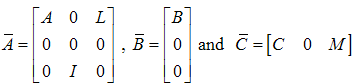
- The system has been assumed to be influenced by additive faults
 in the states and additive disturbance
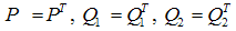
  on the output. The matrices
  and
and  are faults matrices:
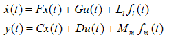 | (1) |
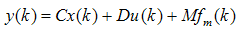
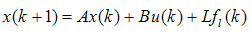
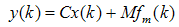
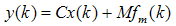
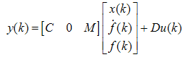
 is a state vector,
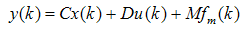
  represents a control input vector,
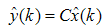
  is a measurement output vector, and F, G, C and D are known constant matrices [4].
2.2. Design a New Optimal Adaptive Diagnosis Observer (OAD)
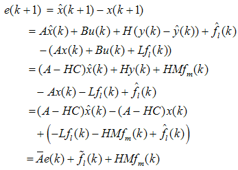
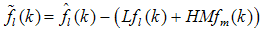
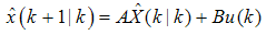
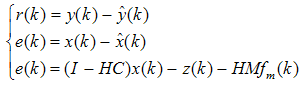
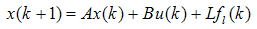
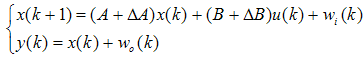
- A new optimal adaptive observer has been implemented to detect and diagnose an additive fault, a sensor disturbance and estimate the states of the plant in (1) as follows:
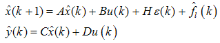 | (2) |
 where it can be found based on the optimal conditions.
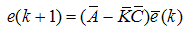
  is assumed to be the residual while
  is the state error defined as:
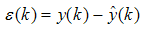 | (3) |
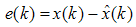 | (4) |
 | (5) |
 ,
, . Therefore, the residual can be rewritten to become:
 | (6) |
 for the system being realized as:
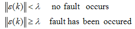 | (7) |
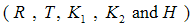
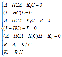
 of the adaptive observer in (2) can be obtained such that the following conditions:
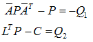 | (8) |
 are positive definite and
  is a Hurwitz. The goal of fault diagnosis is to find a diagnostic algorithm for
  and an observer gain vector
  such that:
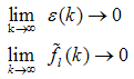 | (9) |
 | (10) |
 which are pre-specified gain matrices and for any
  , there exists
  , yielding:
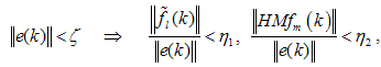 | (11) |
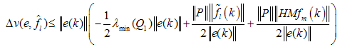
 should be positive definite matrices.Proof of the Theorem: Define the Lyapunov function
  candidate:
 | (12) |
 where
where  . Then:
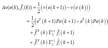 | (13) |
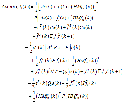 | (14) |
 | (15) |
 | (16) |
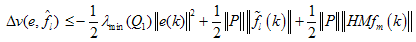
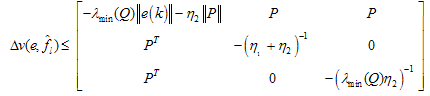
 , no matter how small, there exists
  , yielding:
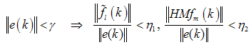 | (17) |
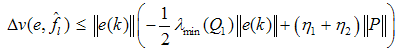 | (18) |
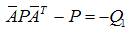
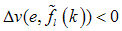 , the linear system is asymptotically stable by Lyapunov stability theorem the condition to be satisfied is:
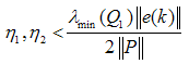 | (19) |
 | (20) |
3. Linear Observers
- Six Known Linear Observers to detect and diagnose the fault are studied and demonstrated. The observers differ in model and method of fault dealing which cover most fault detection techniques. Models of the observers will be introduced as follows:
3.1. Luenberger Observer (LO)
- The plant shown in (21) and (22) is influenced by additive faults
 on states and the additive faults
  on the output. The matrices
  and
and  are faults matrices
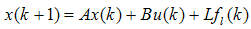 | (21) |
 | (22) |
 and
and  are known constant matrices. The states and output of observer is given by
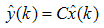
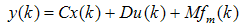
 | (23) |
 | (24) |
 is the gain matrix of the observer, r(k) is the residual and e(k) is the errors between the plant’s states and states of observer.
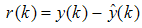 | (25) |
 | (26) |
 | (27) |
 | (28) |
3.2. Kalman Observer (State Estimation Observer) (KO)
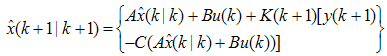
- For the linear system which is represented in (29) and (30) Kalman observer can be formed through the prediction and correction of the states of plant to give
 | (29) |
 | (30) |
 | (31) |
 | (32) |
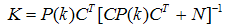 | (33) |
 | (34) |
 | (35) |
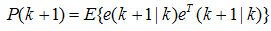
 is the covariance matrix of the estimation error and satisfies the following matrix Riccati equation
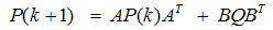 | (36) |
 | (37) |
 is the covariance matrix of the faults on the output
 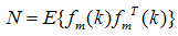 | (38) |
 | (39) |
 | (40) |
3.3. Unknown Input Observer and Robust Fault Detection (UIO)
- The plant in (41) and (42) is influenced by additive faults
 on states and additive faults
  on output, and then the linear system is represented as
 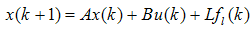 | (41) |
 | (42) |
 in the form of
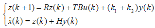 | (43) |
 | (44) |
 | (45) |
 ) as
) as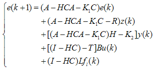 | (46) |
 , this leads to the following conditions
 | (47) |
 | (48) |
 | (49) |
 | (50) |
 using the pole placement method by using
  and assume the observer is stable. The Eigen values of
  are the same of the assumed poles. If all Eigen values of
  are stable,
  will approach to zero asymptotically. Therefore, it is a key to design gains. The assumption is that the matrices
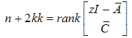
  is of a full column rank (This condition can ensure that (
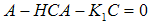 ), so that
 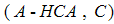 is an observable pair.
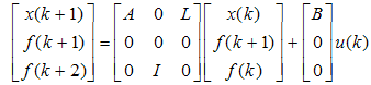
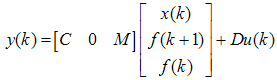
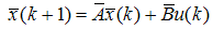
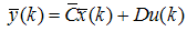
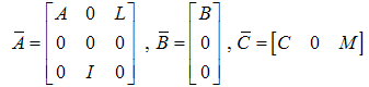
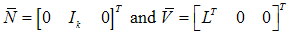
3.4. Augmented Robust Observer (ARO)
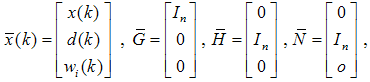
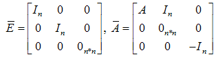
- Let us consider the plant is a linear system which is represented in (51) and (52) as
 | (51) |
 | (52) |
 | (53) |
 | (54) |
 | (55) |
 | (56) |
 | (57) |
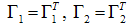
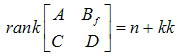
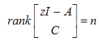
 The stability condition for observer is described in (58). To obtain asymptotically stable observer, a sufficient condition for this is that the pair (
 and
and  ).
). | (58) |
 | (59) |
 | (60) |
 | (61) |
 | (62) |
 | (63) |
 | (64) |
 | (65) |
 is observable. The observer gain can be found using the poles placement method. Since the relationship in (53) is not always true
  and the bounded disturbance signal not affected by the gain parameter therefore needs to other type of observers like high gain observer.
3.5. High Gain Observer (HGO)
- Consider the system as a linear system with faults to be represented as
 | (66) |
 | (67) |
 | (68) |
 | (69) |
 | (70) |
 | (71) |
 | (72) |
 ,
,  The observer is therefore given by
 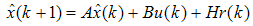 | (73) |
 | (74) |
 | (75) |
 | (76) |
 and µ is less than real parts of all Eigen values of
  . So obtain a stable observer in discrete time model,
  . In our simulation, it has been chosen as
  .2- Find the matrix
  using discrete Lyapunov function:
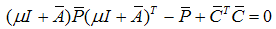 | (77) |
 It can be seen that when µ is increased the matrix P will be decreased. Therefore the observer is robust against the input disturbance and faults.
 3.6. Sensitive High Gain Observer (SHGO)
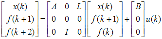
- Let us consider the linear system with multiplicative faults in the parameters and additive faults on the states, the model of the system is given as
 | (78) |

 and
and 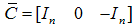 where
where  is the number of states. The observer can be modified as
 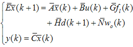 | (79) |
 and
and ) are bounded. The observer can be further modified to give
 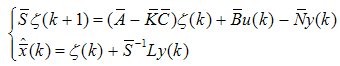 | (80) |
 and
and  are the gain matrices.The following algorithm is implemented to design the gain matrix of observer: 1- Incontinuous time system, choose
  as a positive number where µ is less than real parts of all Eigen values of
  . For discrete time system, µ is chosen to be less than 1 in order to obtain stable observer.In the simulation of a DC motor, a discrete time model is considered, therefore
  and
and  . 2- The Lyapunov function is used to evaluate the matrix
 | (81) |
 Let us assume the following
  and
and 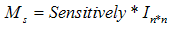 where
where  is a non-singular matrix. One can thus consider
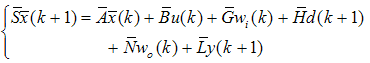
 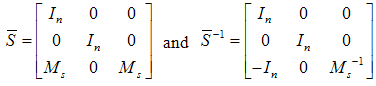 Then it can be further obtained that
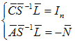 | (82) |
 | (83) |
 | (84) |
 | (85) |
4. Performance Evaluation
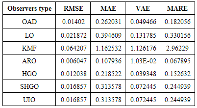
- In order to evaluate fault detection, diagnosis and performance, absolute error and relative error criteria are used. Absolute error is the amount of physical error in a prediction, while relative error gives an indication of how good a prediction is relative to the size of the parameter. Root mean squared error (RMSE), mean absolute error (MAE) and variance absolute error (VAE) are used to calculate absolute error. For relative error, mean absolute relative error (MARE) and variance relative error (VRE) are used. The above statistic formulas list as follows
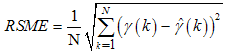 | (86) |
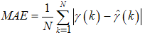 | (87) |
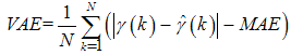 | (88) |
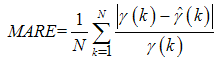 | (89) |
 represent the number of samples, and the measured and desired values respectively.
5. Case Study and Results
5.1. General Model of Continuous Linear DC Servomotor
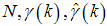
- A DC servomotor is a second order system with multiple inputs and multiple outputs. It has power of
 watts and speed of
  , and the motor has two pairs of brushes and two pole pairs. The model has been obtained according to the parameters of armature resistance, armature inductance, magnetic flux, voltage drop factor, inertia constant and viscous friction. The input signals are the armature voltage
  , which has been represented in simulations codes as a step function, and the torque load
  , which is assumed equal to 0.1. The measured output signals are the armature current
  and the speed of motor
  . The values of the parameters were identified by the well-known least square estimation in the continuous time domain as follows [4]:
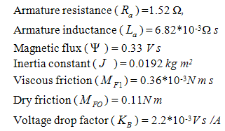 The continuous time model of a DC motor as a state-space form is thus obtained as:
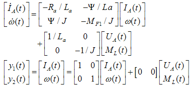 | (90) |
5.2. Comparison with an Additive Fault and Disturbance
- Matlab code has been used to implement the plant (DC servomotor) and the seven discrete time observers
 and
and  with a 0.1 second sample time, where the additive faults have been proposed on the states after 10 seconds and their faults matrices are assumed as:
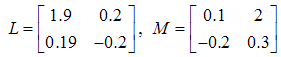 The gain matrix of the observers
  and
and  can be evaluated using the pole placement method. Therefore the poles of discrete observers are chosen as
 respectively. Moreover, the tuning parameter for
  is chosen as
  whereas for
  the parameter is
  and the while the gain matrices for
  are as follows:
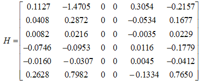 Furthermore, the gain matrix for
  is obtained as follows:
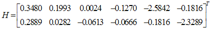 However, the parameters for the adaptive diagnosis, which will verify the conditions in (8), are evaluated as follows:
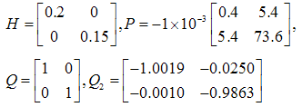 Whereas for the adaptive fault diagnosis, the parameters are:
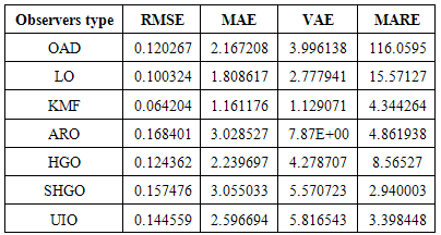
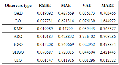
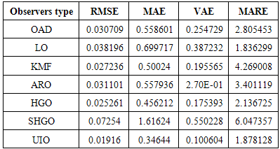
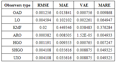
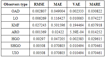
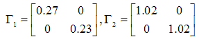 To study the observers’ activity, three types of fault and disturbance are applied to the system: white noise (random with zero mean), coloured noise (randomly with mean) and non-Gaussian noise (randomly sinusoidal noise). The effectiveness of each observer design is tested through comparing the method of the gain matrix design, according to the performance criteria in0. Moreover, Table 1 to Table 3 include the performance values of the first output of the observer, while Table 4 to Table 6 show the performance for the second output of the observers.
|
|
|
|
|
|
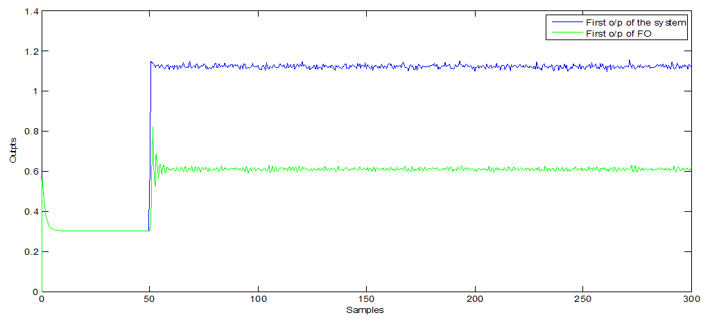
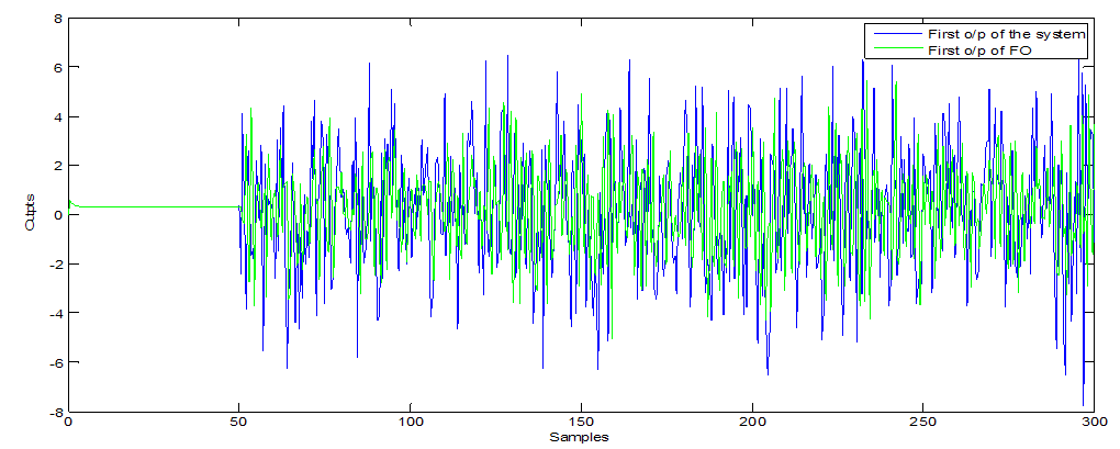 | Figure 1. First o/p ODA observer (with white noise) |
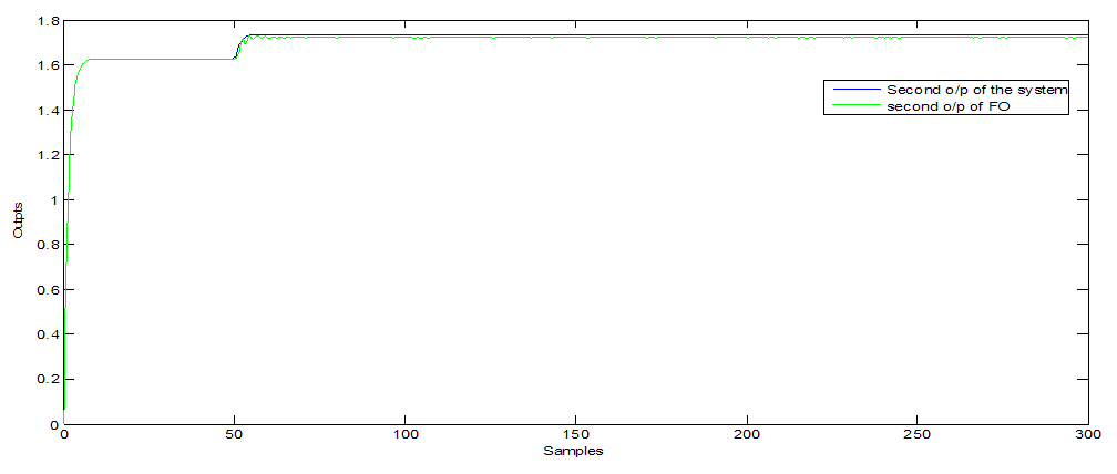
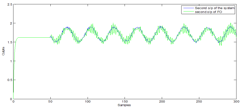
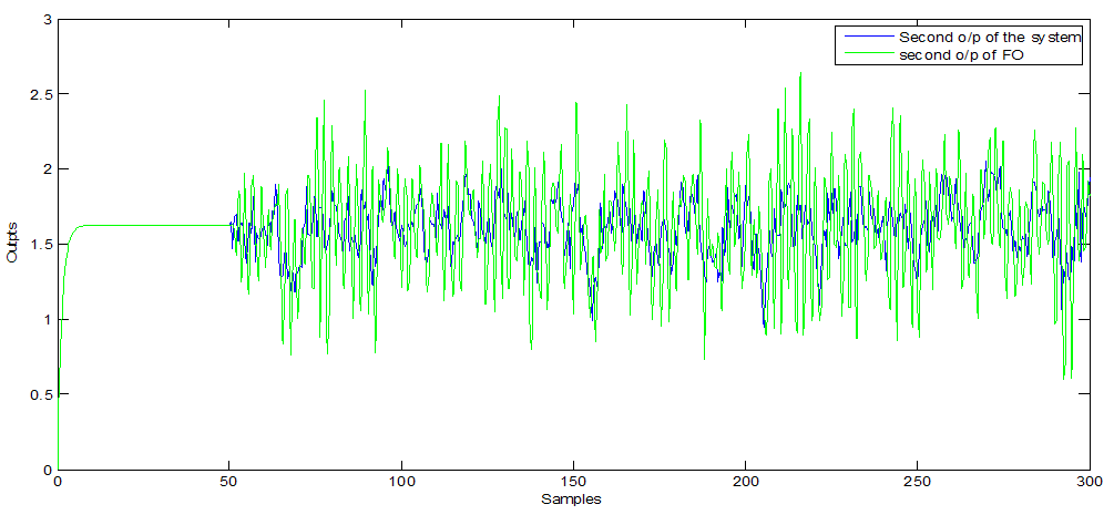 | Figure 2. Second o/p of ODA observer (with white noise) |
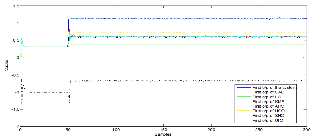
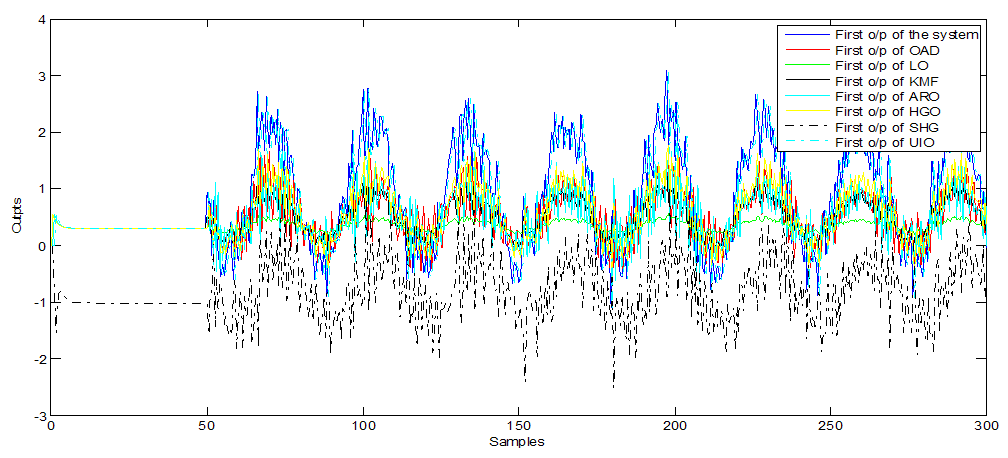
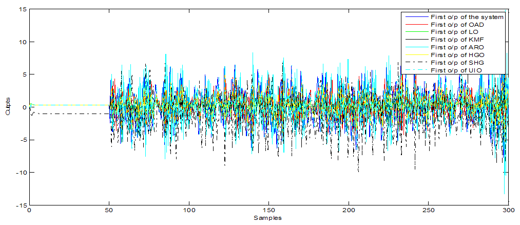 | Figure 3. First o/p of additive fault observers (with white noise) |
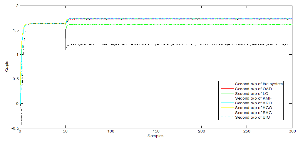
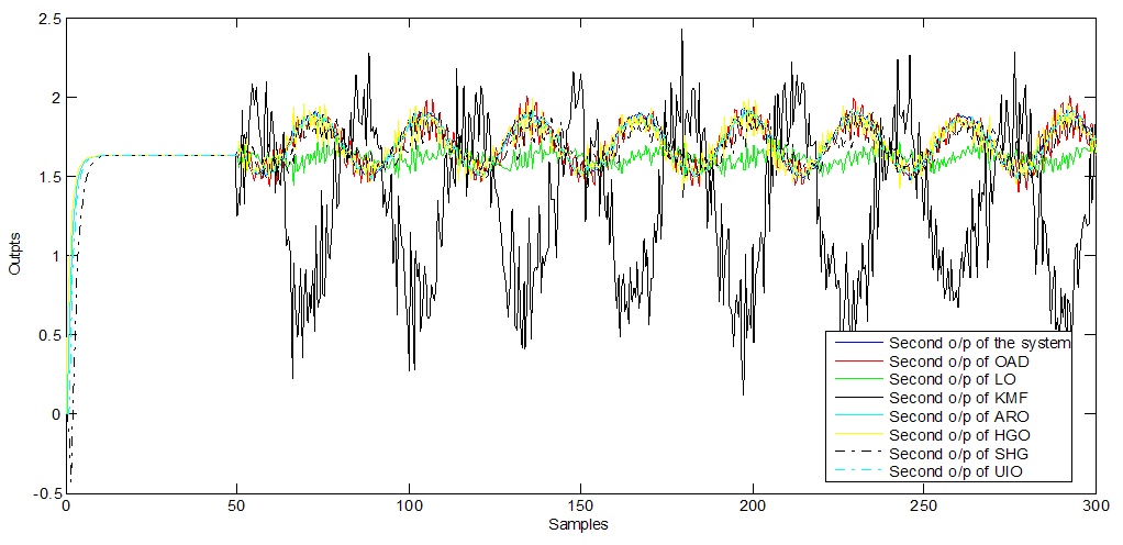
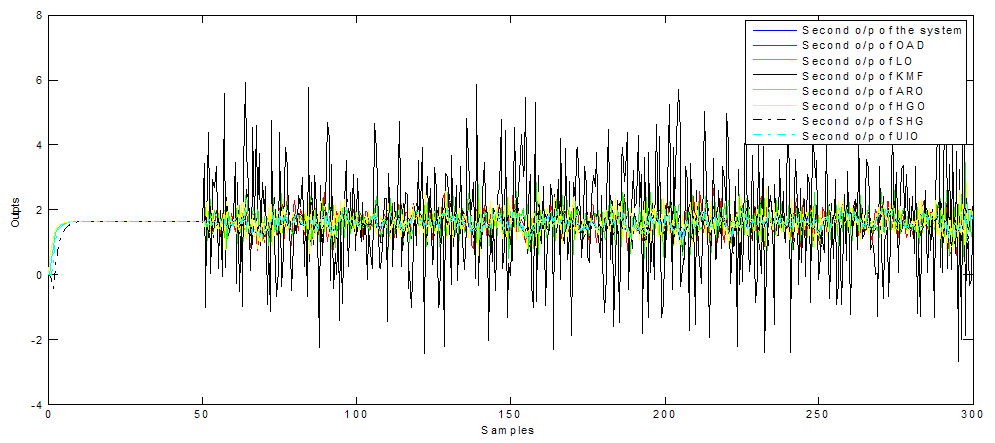 | Figure 4. Second o/p additive fault observers (with white noise) |
 | Figure 5. First o/p of ODA observer (with coloured noise) |
 | Figure 6. Second o/p of ODA observer (with coloured noise) |
 | Figure 7. First o/p of ODA observer (with coloured noise) |
 | Figure 8. Second o/p additive fault observers (with coloured noise) |
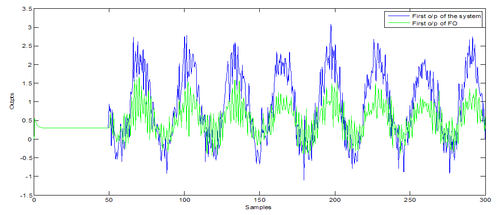 | Figure 9. First o/pof ODA observer (with non-Gaussian noise) |
 | Figure 10. Second o/p of ODA observer (with non-Gaussian noise) |
 | Figure 11. First o/p of observers (with non-Gaussian noise) |
 | Figure 12. Second o/p of observers (with non-Gaussian noise) |
- Furthermore, Figure 1, 5 and 9 show the first output of the observers and Figure 2, 6 and 10 show the second output of the observers. The comparisons are also clear in Figure 3, 7 and 11 for the first outputs while Figure 4, 8 and 12 show the second outputs. The results of the comparisons according to the three types of fault and disturbance show that the new proposed observer OAD can more than compete with the other six good observers
 ; it has the highest performance.
6. Summary
- This paper presents the design of anew optimal adaptive diagnosis observer (ODA) which is designed for additive fault and disturbance; its gain matrix verifies the proposed Lyapunov conditions. In fact, the strategy of a design for dynamic estimated fault for the observer depends on the two positive pre-specified matrices: one tunes the estimated fault and the second matrix tunes the residual between the plant and the observer. In addition, in the presence of disturbance and fault, the performance of the ODA observer is tested through comparing it with six different good linear observers Luenberger Observer (LO), Kalman (Filter) Observer (KO), Unknown Input Observer (UIO), Augmented Robust Observer (ARO), High Gain Observer (HGO), and Sensitive High Gain Observer (SHGO).The assumed disturbance and faults are white noise, coloured noise and non-Gaussian fault. A MIMO DC servomotor has been used as a benchmark in the performance assessments. While the considered criteria of performance are root mean squared error (RMSE), mean absolute error (MAE) and variance absolute error (VAE) and mean absolute relative error (MARE). However, the comparison results of the ODA with the six other good observers show that it is the best overall where it has a high ability to detect and diagnose different fault and disturbance type as well as it is the best in states estimation performance.