1. Introduction

Studying fluid flow characteristics is vital for designing more efficient combustors. Many methods have been used to realize an efficient design (e.g., one major way is achieved by reducing emissions of undesired products, such as NOx, CO and unburned hydrocarbons). Recently, designers have used swirlers to generate a swirl flow inside the chamber to get a reversal flow that entrains and recirculates a part of combustion products in order to be mixed with the fuel and incoming air. A swirling fluid flow is created when a spiral motion is formed along its axial axis; it causes a complex three dimensional flow. This swirl phenomenon is studied because of its importance in increasing combustion efficiency. In addition, it minimizes combustors’ sizes since it reduces flame length and enhances the stability of the flame and gives better mixing between fuel and oxidizer thus achieving uniform pattern factor.

Turbulent swirling flows have highly complex, three-dimensional, unsteady flow fields which include reverse flow regions. Therefore, they have been the subject of many experimental, numerical and theoretical investigations and have been reviewed extensively in the literature during the last five decades (see for example [1-12]). Most of the studies are based on experimental results using several types of sensors and actuators tomeasure velocities, forces and pressures on several coordinate locations. Particle image velocimetry (PIV) and laser Doppler anemometry/velocimetry are some of the techniques used to measure swirl flow field velocity components.

Turbulent swirling flows modelling remains a challenge in fluid mechanics and a large body of literature has been published to deal with various flow configurations (confined and unconfined, reacting and non-reacting) and/or specific phenomena such as flow structure and instabilities, and/or vortex breakdown. A comprehensive treatment on swirl flows can be found in the book by Gupta and Liley[2].

The axisymmetric sudden expansion geometry is relevant to many swirling applications, particularly swirl burners and combustors. Sudden expansion flows combine geometric simplicity with complex flow features such as separation and reattachment. They share many similarities with the flow past a backward facing step (i.e., the existence of three distinct flow regions: recirculation, reattachment and redevelopment). The reverse flow region size is an important feature of sudden expansion flows and it depends on swirl strength and type (e.g., free/forced vortex or constant angle), Reynolds number, expansion ratio, and free stream turbulence (for example, see[3-10]).

The structure of swirling flows is very sensitive to the way the swirl is introduced (i.e.; the inlet conditions). The effects of inlet or initial swirl profile and expansion angle on the characteristics of the swirling flow were investigated by Nejad and Ahmed[4]. They introduced swirl by three different types of swirlers: free vortex, forced vortex and constant angle, respectively. They showed that there are significant differences in the flowfield and turbulence characteristics when a different swirler is employed. In their study, for the same swirl number, a central recirculation was only observed in the case of free vortex type of swirling flow after the expansion. However, the centreline turbulence levels were the greatest for constant-angle swirling flow due to the large motion of the vortex centre precession.

Hallett and Toews[5] showed that a lower velocity near the axis or a reduced radius of the solid body vortex core in the inlet will reduce the critical number required for central recirculation. An increase in the expansion ratio up to 1.5 will also reduce the critical swirl number. For expansion ratios greater than 1.5, either a reduction or an increase of the critical swirl number is reported, depending on inlet conditions.

Because of the limited (discrete) data provided by such techniques, however, an interpolation tool should be utilized to precisely implement the turbulence statistics. A new methodology has to be considered to provide enough set of information. Artificial Neural Networks (ANN) analysis is suggested to predict turbulence statistics and to enlarge the experimental data, therefore, enhancing dump combustors design.

2. Literature Review

Artificial neural networks are one of the artificial intelligence concepts that have proved to be useful in various engineering applications[13-23]. Their greatest advantage is in their ability to model complex non-linear, multi-dimensional functional relationships without any prior assumptions about the nature of the relationships. The network is built directly from experimental data by its self-organizing capabilities and can therefore be considered as a black box and it is unnecessary to know the details of the internal behavior. These nets may therefore offer an accurate and cost effective approach for modeling engineering problems. ANN have already been used in medical applications, image and speech recognition, classification and control of dynamic systems, prediction of mechanical properties of materials among others[17-23]; but only a few studies have used them in swirl flow velocity field reconstruction[13-16]. Pruvost et al.[13] used ANN to determine hydrodynamical parameters obtained using particle image velocimetry (PIV) on the entire geometry of an annular test-cell involving a swirling decaying flow. They concluded that this method reduces the investigation time through reducing the number of needed experimental measurements while leading to a better understanding of the flow field by establishing pertinent hydrodynamical parameters.

Ghorbanian et al.[14] used a general regression ANN to optimize the design of pressure-swirl injectors.Measurements obtained from Phase Doppler Anemometry (PDA) measurements of the velocity distributions were used to train the network. The model used was shown to accurately reconstruct the velocity flow field of a single swirl spray as well as the interaction of two sprays. Ahmed and El Kadi [15,16] used generalized feed forward network to predict the flowfield characteristics downstream of a sudden expansion dump combustor model. The results obtained for free vortex swirler (S = 0.4) indicated that generalized feed forward network is capable of predicting the mean velocity components and the turbulence intensities of the velocity components.

The general objective of the current study is to report detailed experimental database to help in the understanding of the behavior of axisymmetric, recirculating, and incompressible turbulent flows. Because the obtained velocity-field is not continuous and the acquisition area remains limited, a complete investigation of the flow field would request numerous measurements. Thus, an extensive experimental investigation would be expensive and require a very long time to obtain sufficient data. Since ANN can deal with non-linear modeling, they seem to be an efficient tool for the reconstruction of data linked to multiple parameters, and thus an interesting alternative solution to common interpolation schemes. To evaluate the accuracy of the different networks, a large set of flowfield characteristics downstream of a sudden expansion dump combustor model (measured using laser Doppler velocimetry) is used. Earlier results obtained by Ahmed and El Kadi[15,16] for free vortex swirler (S = 0.4) indicated that ANN are capable of predicting the mean velocity components and the turbulence intensities of the velocity components.

In this study, the turbulence statistics are predicted for a constant angle swirler (S = 0.5) using several ANN architectures and are compared to obtain the best network that could be used in this problem.

3. Experimental Facilities

3.1. Combustor Design

The model where data is captured consists of two major parts; an inlet assembly and a combustion chamber. The inlet assembly contains a settling chamber of 300 mm diameter, a Plexiglas inlet pipe with 2850 mm length and 101.6 mm inner diameter, and a cylindrical Teflon swirler housing that has 104.5 mm inner diameter, 152.4 mm outer diameter, and 154 mm in length. A distinctive characteristic of this model is its capability of dump plane (swirler housing) positioning with respect to the plane of measurement inside the combustion chamber. This is accomplished by supporting the entire inlet assembly on a traversing mechanism controlled by a stepper motor. The inlet average velocity is monitored with a flow meter located far upstream of the swirler housing, and maintained at average velocity corresponding to Reynolds number of 1.5x10⁵. This velocity is high enough to ensure a turbulent flow in the combustor.

The combustion chamber itself contains a Plexiglas tube with 152.4 mm inner diameter and 1850 mm in length, terminating into a larger pipe (exhauster). The measurement station is designed to accept different window assemblies. One is designed to provide optical access for LDV traversing in the horizontal plane (see Figure 1).

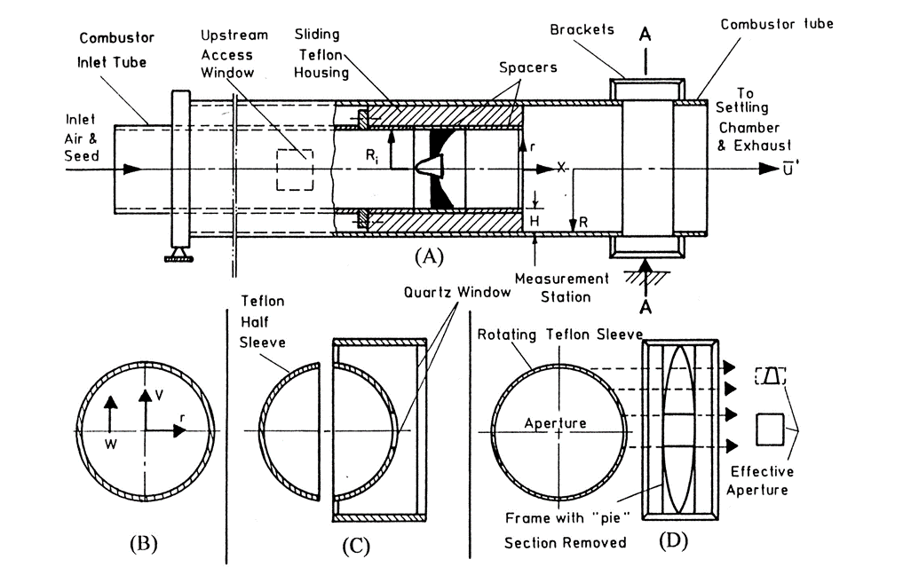Figure 1. Schematic of the experimental set-up; (A) Dump combustor model; (B) Section A-A; (C) Assembly for measurements in the horizontal (U-V) plane; (D) Assembly for measurements in the vertical (U-W) plane

The swirler is at a constant angle type, similar to the one used by Ahmed and Nejad[24]. The current facility employed a swirler that has 12 curved vanes. Swirler dimensions are 19 mm inner diameter (central hub) and 101.6 mm outer diameter.

3.2. Measurements Techniques

The measurements of velocity are performed using a TSI Inc. 9100-7 four-beam, two-color, back scatter fiber-optic LDV system. It has two TSI 9180-3A frequency shifters to provide directional sensitivity. The entire optics is mounted on a three-axis traversing table with a resolution of ±2.5 µm. The system is configured so that the fringe inclinations are at 45.67º and 134.17º to the combustor centerline. The approximate measurement volume dimensions based on intensity points are 390 µm length and 60 µm width.

The photomultipliers signals were processed by two TSI burst counters - models 1990 B\C with low pass filters, set at 20 MHz, and high pass filters set at 100 MHz on each processor. Calculations of statistical moments from standard formulae were done at each measurement location using double precision data (48 bit). The problem of velocity bias in LDV measurements was corrected in this study by the use of the time between individual realizations as a weighing factor (interarrival bias correction techniques, see Ahmed[10]).

The swirl number is 0.5, the measured profiles are located at x/H=.38, 1, 2, 3, 4, 5, 6, 8, 10, 12, 15, and 18. At each profile, the radial coordinate changes from 0 to 3 with a step size of 0.1. The purpose of this study is to test the ability of neural network in implementing such a model and compare the results obtained from the network with the experimental data.

4. Artificial Neural Networks

Artificial neural networks can generally be defined as a structure composed of a number of interconnected units called neurons[25]. Each neuron has an input/output (I/O) characteristic and implements a local computation or function. The output of each neuron is determined by its I/O characteristic, its interconnection to other neurons and (possibly) external inputs, as well as its internal function (see Figure 2). The network usually develops an overall functionality through one or more forms of training. As in nature, some of the neurons interface with the real world to receive its input (input layer), while others provide the world with the network’s output (output layer). All remaining neurons are hidden (hidden layers). Each input to a neuron has a weight factor that determines the contribution of this neuron to the whole network. In addition, it has a bias term, a threshold value that has to be reached or exceeded for the neuron to produce a signal, a nonlinearity function that acts on the produced signal, and an output. Learning is the process by which the neural network adapts itself to a stimulus and eventually (after adjusting its synaptic weights) produces the desired response. Many publications discuss the development and theory of ANN (for example, see references[25-27]).

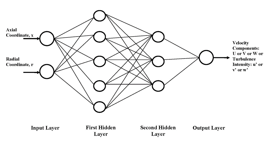Figure 2. General configuration of artificial neural networks

In this study, the predictions obtained using 3 neural networks architectures are compared to determine the type of network that best predicts the velocity profiles. The networks used here are: the generalized feed forward (GFF), the radial basis function (RBF), and the coactive neuro-fuzzy inference system (CANFIS).

4.1. Generalized Feed Forward Network

Multilayer feedforward ANN with backpropogation training have been the most popular and commonly used because of their adequate generalizing capabilities. However, they could suffer from some drawbacks such as local convergence and the need for large training cases in order to make adequate generalization. Therefore other types of neural networks such as RBF are considered to overcome such problems and other problems the training data may have.

In this network, neurons in the input layer act as buffers for distributing input signals to neurons in the hidden layer. Each neuron in the hidden layer gets its value by summing up the input signals after weighting them with weighting factor thus the output can be written as[28]:

(1)

4.2. Radial Basis Function Network

He RBF is a classification and functional approximation paradigm developed by M.J.D. Powell[29]. These networks are non-linear hybrid networks usually containing a single hidden layer. The hidden layer consists of locally tuned units, where the response is localized and decreases as a function of inputs distances from the unit’s center. The output layer consists of linear units in most cases[29]. It is claimed that these networks learn faster than the MLP and need less number of training data, their generalization capabilities is however limited.

Usually, a hidden layer in RBF network employs a Gaussian activation function, which can be described by:

(2)

Where corresponds to the weight of the unit and is called the net activation. These weights are used with Gaussian function to determine the center of units. The centers and widths of the activation functions are obtained by unsupervised learning while supervised learning is used to update the connection weights between the hidden and output layers. Note that the units have maximum net activation, which means a maximum output value occurs when this shows that the sensitivity of units depends on distance.

The output units are implemented linearly, where:

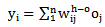(3)

Where is the output of the previous hidden layer neurons, is the weight of the interconnection between the last hidden layer and the output layer.

It is recommended to use the RBF network when the system model has a radial tendency, in other words, the model behaves always towards the center of the system.

4.3. Coactive Neuro-Fuzzy Inference System Network

This network is a combination between classification and regression trees (CART) and the adaptive neuro-fuzzy inference system (ANFIS) in a two step procedure. CART is a tree-based algorithm used to optimize the process of selecting suitable predictors from a large set of predictors. Using the selected predictors, ANFIS builds a model for continuous output of the predictions[30-32].

The fundamental component for CANFIS is a fuzzy neuron that applies membership functions (MFs) to the inputs. Two membership functions commonly used are general Bell and Gaussian[33]. The network also contains a normalization axon to expand the output into a range of 0 to 1. The second major component in this type of CANFIS is a modular network that applies functional rules to the inputs. The number of modular networks matches the number of network outputs, and the number of processing elements in each network corresponds to the number of MFs. CANFIS also has a combiner axon that applies the MFs outputs to the modular network outputs. Finally, the combined outputs are channeled through a final output layer and the error is back-propagated to both the MFs and the modular networks.

The CANFIS neuro-fuzzy modular network computes a weighted sum of the outputs of a certain number of MLPs, this leads to optimize all the parameters by minimizing the sum over all data of squared errors[34].

5. Results and Discussion

5.1. Influence of Network

The target of this study is to find out the neural network structure that most accurately predicts the velocity components and the turbulence intensities at the different locations. The input parameters of the network are the x and r coordinates, while the non-dimensional mean axial and tangential velocities (U and W) and the turbulence intensity components are the possible outputs from the network. Rather than having one complex neural network to predict all the velocity components and turbulence intensities, a simpler network was used to separately predict each parameter. NeuroSolutions 5 software package[35] is used to construct, train and test the networks.

The effect of varying the transfer function and learning algorithm on the accuracy of the predictions was investigated in[36]. Here, the results presented have all been obtained using a tanhaxon transfer function with a Levenberg- Marquardt learning algorithm[37-39]. For all the cases considered, the network is trained five times using all but one of the velocity or turbulence intensity distributions obtained experimentally at different values of x to overcome the effect of the initial guess. These networks were then tested by comparing the predicted results obtained from the ANN to the experimental results of the profile not used in training. Once we are confident of the accuracy of the network, one can use it to predict the velocity and turbulence intensity distributions at any location, x, for which no experimental data is available. Selecting the most appropriate network is based on evaluating the correlation coefficient (cc) and the normalized mean square error (NMSE), which are defined in equations (4) and (5), respectively,

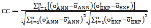(4)

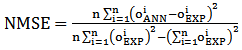(5)

where is the output from the neural network at each coordinate is the experimental value of the parameter at the same coordinate. 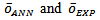are the average predicted and experimental results, respectively, and is the number of data points used in testing (exemplars). The results shown next are obtained using the following properties of the three neural networks considered:

• For the GFF network, one hidden layer was used; the maximum number of epochs was set at 2000; and the number of processing elements was varied between 9 and 20.

• For the RBF network, one hidden layer was also used; the competitive rule used is Conscience Full with Euclidean metric system[29]; the maximum number of epochs used in unsupervised and supervised learning was set to 500 and 1000 respectively; and the number of cluster centers was varied between 10 and 20.

• For the CANFIS network, the Takagi-Sugeno-Kang (TSK)[31] fuzzy model with Bell and Gaussian membership functions[32] was used; the maximum number of epochs used in supervised learning was set to 250; and the number of membership functions was varied between 3 and 10.

As mentioned before, the selection of the most efficient network is based on calculating the average correlation coefficient obtained after training the network at all-but-one value of x. The network is then tested for the untrained value of x; the value of the correlation coefficient obtained is referred to as the testing correlation coefficient.

Figures 3-6 show the average testing correlation coefficients for all networks at x/H = 3, 6, 10 as a function of number of processing elements for GFF network, number of membership functions for CANFIS networks (Bell and Gaussian models), and number of clusters for RBF network for non-dimensional 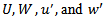respectively.

The best predictions obtained using the GFF network (Fig. 3) for non-dimensional 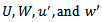are obtained when the number of neurons is 19 for U, and 18 neurons for all of with correlation coefficients of 0.966, 0.997, 0.985 and 0.944, respectively.

Figure 3. Average cc of testing GFF network for non-dimensional at x/H=3, 6, 10 as a function of number of neurons

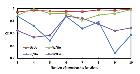
Using the RBF network (Fig. 4), the highest correlation coefficients for were obtained with 13, 19, 16, and 16 clusters, respectively, with corresponding cc values of 0.889, 0.936, 0.688 and 0.617. The maximum correlation coefficients for the Gaussian-based fuzzy model (Fig. 5) forwere found to be 0.989, 0.995, 0.875, and 0.877, respectively at 10, 4, 3, and 6 membership functions. For the bell-based fuzzy model (Fig. 6), the highest correlation coefficients for 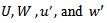were 0.989, 0.995, 0.694, and 0.966, respectively at 9, 7, 3, and 8 membership functions.

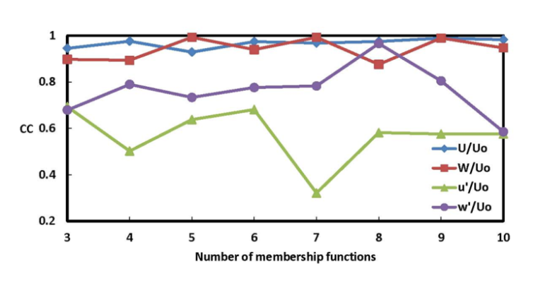Figure 4. Average cc of testing Bell CANFIS network for non-dimensional at x/H=3, 6, 10 as a function of number of membership functions

Figure 5. Average cc of testing Gaussian CANFIS network for non-dimensional at x/H=3, 6, 10 as a function of number of membership functions

Figure 6. Average cc of testing RBF network for non-dimensional at x/H=3, 6, 10 as a function of number of cluster size

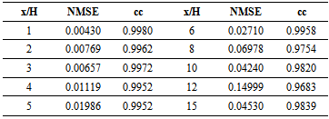
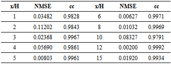
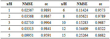
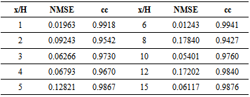
These results show that, on average, GFF networks produce the best predictions for all of velocity and turbulence intensity components, while the Gaussian-based fuzzy model gives more accurate predictions than fuzzy model with bell membership functions for and RBF networks fail to give accurate results at any number of clusters. On that basis, the use of GFF networks to predict the velocity and fluctuating velocity profiles.

The generalized feed forward network will now be used to predict the velocities and turbulence intensities distributions obtained at values of x not used in training the network and compare these predictions to the experimental data.

Table 1 shows the NMSE and cc values obtained when predicting the axial velocity using a GFF network with one hidden layer with 19 neurons. These results shows that, even at the lowest correlation factor (0.9683) obtained at x/H=12, the network accurately predicts the axial velocity.

Similarly, Tables 2, 3, and 4 show the NMSE and cc values at each profile for the tangential velocity component, the tangential turbulence intensity, respectively. The network used in this case is a one-hidden layer GFF with 18 neurons. Table 2 shows that the tangential velocity component profiles are more accurately predicted compared to the axial ones (Table 1) since the lowest correlation coefficient obtained (0.9791) is higher than that obtained for the axial case.

The values listed in Table 3 show that the GFF network is unable to accurately reconstruct the last two axial turbulence intensity profiles (i.e. x/H=12 and 15). This could be due to the different shapes of these profiles compared to those at other locations.

The NMSE and cc obtained when predicting the tangential turbulence intensity profiles are shown in Table 4. The NMSE values obtained here are the lowest compared to all other components.

Table 1. NMSE and cc Values as a Function of x/H for Axial .Velocity Profiles

Table 2. NMSE and cc Values as a Function of x/H for Tangential Velocity Profiles

Table 3. NMSE and cc Values as a Function of x/H for Axial Turbulence Intensity Profiles

Table 4. NMSE and cc Values as a Function of x/H for Tangential Turbulence Intensity Profiles

5.2. Comparison between Experimental and Network Velocity Profiles

Figures 7-10 illustrate the comparison between the three networks and the experimental data at x/H=1, 3, 5, and 8. The experimental data are shown as open circles markers, the predictions done by the GFF network are plotted as solid red lines, RBF network data are presented as dashed green lines, and the CANFIS predictions are displayed as dashed-dotted blue lines.

The plots show that GFF is the most accurate network between the three networks considered. The graphs clearly show that GFF network successfully predicts most of the profiles with better trend than RBF or Gaussian CANFIS networks. Thus, GFF network is recommended to reconstruct turbulence statistics for this combustor model. Detailed results of the flow field utilizing GFF will be presented in a separate paper.

The mean non-dimensional velocity profiles are shown in Figures 7 and 8. GFF shows the recirculation zones at the corners and around the center line. Figures 9 and 10 show the turbulence intensities distributions at various values of the distance x. It is obvious that two peaks characterized the swirling flow around the inner and outer shear layers (i.e., the larger is seen in the boundaries of CTRZ, and the smaller occurred in the shear layer of CRZ). Turbulence activities are gradually reduced downstream of the reattachment point. It is interesting to note that the peak value of axial turbulence intensities is observed to move towards the combustor wall as it decays in strength and grows in size, indicating a progressive development of the outer shear layer. Turbulence activity is seen to be more concentrated in the central shear layer and the centers of the maximum values, for the two regions are located approximately at x / H = 3.0 .

In the tangential direction, the flow did not completely recover near the core (due to the existence of CTRZ) as indicated by relatively higher values of stresses at each axial location, and downstream of x / H = 8.

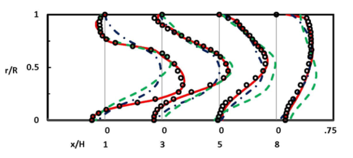Figure 7. Evolution of for experimental and neural networks predictions

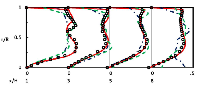Figure 8. Evolution of for experimental and neural networks predictions

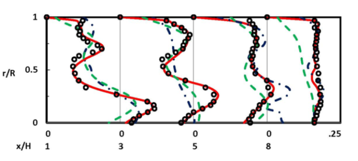Figure 9. Evolution of for experimental and neural networks predictions

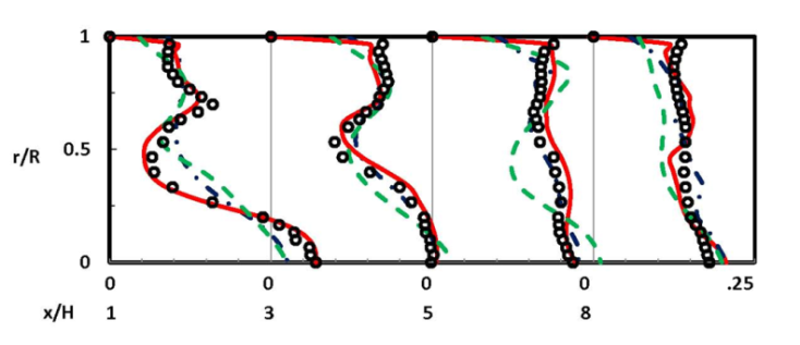Figure 10. Evolution of for experimental and neural networks predictions

6. Conclusions

The experimental data of turbulent swirling flowfield characteristics at a constant swirl number are obtained using two-component LDV and compared with the results obtained from three artificial neural networks architectures. This study of velocity-field reconstruction shows precise predictions of ANN in general and GFF network in particular.

The successful predictions obtained using neural networks encourage producing more data and enhancing the ability of a better combustor design.

ACKNOWLEDGEMENTS

The authors wish to acknowledge the financial support of AUS and also utilizing the various facilities in the preparation of the manuscript.

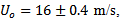
Nomenclature

ANN: Artificial Neural Network

BP: Back propagation

CANFIS: Coactive Neuro-Fuzzy Inference System

CC: Correlation Coefficient

EXP: Experimental

GFF: Generalized Feed Forward

H: Step height

LDV: Laser Doppler Velocimetry

NMSE: Normalized Mean Square Error

o: Previous layer output

r: Radial coordinate

R: Combustor radius

RBF: Radial Basis Function

U: Fluid mean axial velocity

U_o: Upstream fluid mean axial velocity

u’: Root Mean Square RMS of fluctuating component of axial velocity

w’: Weighting factor

W: Fluid mean tangential velocity

w’: Root Mean Square RMS of fluctuating component of tangential velocity

x: Axial coordinate

y: Neural network output