B. Andersson1, V. Golovitchev2, S. Jakobsson1, A. Mark1, F. Edelvik1, L. Davidson2, J. S. Carlson1
1Fraunhofer-Chalmers Centre, Chalmers Science Park, Göteborg, 41288, Sweden
2Department of Applied Mechanics, Chalmers University of Technology, Göteborg, 41296, Sweden
Correspondence to: B. Andersson, Fraunhofer-Chalmers Centre, Chalmers Science Park, Göteborg, 41288, Sweden.
| Email: |  |
Copyright © 2012 Scientific & Academic Publishing. All Rights Reserved.
Abstract
The Rotary bell spray applicator technique is commonly used in the automotive industry for paint application because of its high transfer efficiency and high-quality result. The bell spins rapidly around its axis with a tangential velocity at the edge in the order of 100 m/s. The paint falls off the edge and enters the air with a large relative velocity, driving the atomization into small droplets where the resulting size distribution depends on the process conditions. Especially the rotation speed of the bell is an important parameter governing the size distribution. The main research question in this work is to investigate if the Taylor Analogy Breakup (TAB) model can be used to predict the resulting droplet size distributions in spray painting. As the paint is a viscous fluid a modification of the TAB model taking non-linear effects of large viscosity into account is proposed. The parameters in the breakup model are tuned by optimization to match droplet size distributions obtained in CFD simulations with measured ones. Results are presented for three cases with rotation speeds from 30 to 50 thousand RPM where the full droplet size distributions are compared with measurements. Good results are obtained for all three cases where the simulated size distributions compare well to measurements over a wide range of droplet sizes. The TAB method is able to quantitatively predict the result of the breakup process and can be used in a preprocessing stage of a full spray painting simulation, thereby reducing the need for costly and cumbersome measurements.
Keywords:
Breakup, CFD, Multiphase Flow, Coating, Weber number, Ohnesorge Number
Cite this paper: B. Andersson, V. Golovitchev, S. Jakobsson, A. Mark, F. Edelvik, L. Davidson, J. S. Carlson, A Modified TAB Model for Simulation of Atomization in Rotary Bell Spray Painting, Journal of Mechanical Engineering and Automation, Vol. 3 No. 2, 2013, pp. 54-61. doi: 10.5923/j.jmea.20130302.05.
1. Introduction
In the automotive industry paint primer, color layers and clear coating are sprayed either with classical Pneumatic spray guns or using the Electrostatic Rotary Bell Sprayer (ERBS) technique. The focus here is on the rotating bell technique where paint is injected at the center of a rotating bell and is atomized at its edge. An image of an active bell is shown in Figure 1.The droplet size distribution of the spray determines its characteristics of how it reacts to the external forces applied by the air and the electrostatic field: large droplets tend to travel in straight lines and small droplets follow the force field closely. It is therefore important to have good knowledge about which distribution of sizes there is within the spray to be able to perform spray painting simulations with high accuracy. If a better understanding is gained on how the process parameters affect the distributions this can also be used to tune the result in order to have a better painting result and higher transfer efficiency.Breakup has been studied in many contexts and most extensively within combustion engine research. In a modern diesel or gasoline engine the fuel is injected through a nozzle with high pressure causing the atomization. The TAB model[1] was originally derived for simulation of diesel injection where the penetration depth of the fuel and the average droplet size were compared to measurements. The model has since then been included in several software packages such as KIVA[2] and OpenFOAM[3].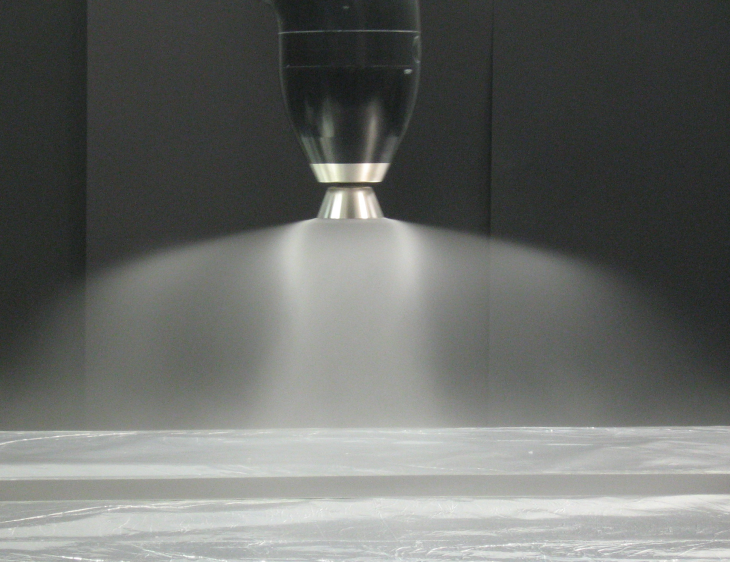 | Figure 1. Photograph of rotary bell spraying towards a target. The actual bell is the cone shaped part at the tip of the applicator head. Courtesy of Swerea IVF |
The aim of this paper is to investigate the ability of the TAB model to predict the paint size distributions by varying the process parameters. The model is implemented in the flow solver IBOFlow[4] which is part of the larger solver framework IPS Virtual Paint used to simulate the spray painting with the rotary bell technique in the automotive industry[5]. By being able to simulate the droplet breakup the need for costly and cumbersome measurements is reduced. The size distributions are then used as input in spray painting simulations for prediction of the paint thickness. In the automotive industry these simulations can be used in the product preparation to reduce the time required for introduction of new car models, reduce the environmental impact and increase the quality.
2. Method
2.1. Taylor Analogy Breakup (TAB) Model
The Taylor Analogy Breakup (TAB) model[1] is based on the fundamental mode of oscillation of a sphere. The sphere is modeled as a damped harmonic oscillator, where the driving force is the relative motion to the surrounding medium, the restoring force is the surface tension, and the damping comes from the viscosity of the fluid inside the droplet. The reader is referred to the original paper[1] for a complete derivation, but some steps are reproduced here.The equation for a damped harmonic oscillator can be written as | (1) |
where  is the displacement of the equator of the droplet from its equilibrium position,
  is the droplet mass,
  is the driving force,
  is the spring constant, and
  is the damping coefficient. The Taylor analogy identifies the following relations for the coefficients,
 | (2) |
where  and
and  are the gas and liquid densities, respectively,
  is the modulus of the relative velocity between the droplet and the surrounding medium,
  is the droplet radius,
  is the surface tension, and
  is the liquid viscosity.The three expressions are derived from the dynamic pressure, the surface tension force and the viscous force, respectively. The dynamic pressure is expressed as
  and is integrated over the projected area of the droplet resulting in a full expression for the force proportional to
  . The pointwise magnitude of the surface tension force is proportional to
  and it is acting on the surface of the droplet giving a total force proportional to
  . The viscous force is proportional to
  and is integrated over the volume of the droplet adding an additional factor of
  resulting in an expression for the force proportional to
  . A constant is assigned to each term that accounts for the omitted constants in the above considerations and to allow for matching the model to measured data.The oscillation amplitude,
  , is made dimensionless by relating it to the droplet radius,
 | (3) |
where  is chosen such that the droplet breaks when
  exceeds unity.By inserting Equations (2) and (3) into Equation (1) a dimensionless equation for the oscillation is obtained,
 | (4) |
By assuming a constant relative velocity  the equation can be solved, giving
 | (5) |
where | (6) |
and  and
and  are the initial conditions for the amplitude of the oscillation and its derivative, respectively. In this work they are both assigned to the value 0.Note that the Weber number,
  , is defined here with the droplet diameter rather than the radius as in the original paper[1].
2.1.1. Large Viscosity Modification
The stability limit of a low viscosity droplet has been determined experimentally to be  . For viscous fluids it is larger and the effect of viscosity on the stability limit has been studied by Brodkey[6]. He came up with an empirical relation taking the viscosity into account by introducing the Ohnesorge number,
 | (7) |
a dimensionless number relating the viscous force to the inertial and surface tension forces. Brodkey's empirical relation is expressed as | (8) |
We see that in the limit of small Ohnesorge numbers, valid for approximately  , the above value of the critical Weber number is recovered. In viscous fluids, however, we see that the stability limit is increased and scales as
  in the asymptotic limit. What is more interesting, perhaps, is that the Ohnesorge number introduces the droplet diameter in the stability criterion. That is, smaller droplets appear more stable than larger ones when exposed to the same Weber number. The scaling of the stability limit with the size of the droplet is
  in the asymptotic limit.Following Schmehl et al.[7] an effective Weber number is introduced, written as
 | (9) |
This effective Weber number is used instead of the regular one in Equation (6) when simulations are performed with the modified TAB model.
2.1.2. Breakup Event Modeling
There are now three free parameters that need to be determined:  ,
,  and
and  . In addition, the size of the resulting droplets of a breakup event needs to be modeled. To do this, a balancing of energy before and after the breakup event is performed. In the frame of reference of the droplet the available energy before the breakup is the sum of the contributions from the surface tension and from the oscillating motion. It is assumed that child droplets are not oscillating immediately after the breakup so that their energy is stored only in the surface tension. Together with the mass conservation constraint this gives an equation for the number of child droplets and their radius. A distribution of droplet radii seems more physically plausible, and therefore the child droplet radius is drawn from a Rosin-Rammler[8] distribution centered at the radius obtained as described above. This gives us two more parameters to be determined: the scale and shape parameters of the distribution,
  and
and  .
.
2.2. Flow Solver
The motion of an incompressible fluid is modeled by the Navier-Stokes equations, | (10) |
 | (11) |
where  is the fluid velocity,
  is the fluid density,
  is the pressure,
  is the dynamic viscosity, and
  is the droplet source term. If two-way coupled simulations between air and paint flow are being performed, the source term for the air flow is equal to the droplet drag force given in Equation (13) below. If one-way coupled simulations are performed the source term for the air vanishes. IBOFlow (Immersed Boundary Octree Flow Solver) uses the finite volume method to solve the Navier-Stokes equations. The equations are discretized on a Cartesian octree grid that can be dynamically refined and coarsened. It is automatically generated and enables adaptive grid refinements to follow moving objects. The Navier-Stokes equations are solved in a segregated way and the SIMPLEC method is used to couple the pressure and the velocity fields[9]. All variables are stored in a co-located arrangement and the pressure weighted flux interpolation is used to suppress pressure oscillations [10]. The Backward Euler scheme is used for the temporal discretization and an adaptive fluid time step is employed such that the maximum Courant number based on the fluid velocity and the movement of the applicators is restricted. Further, the hybrid immersed boundary method[4] is used to model the presence of moving solid objects, without the need of a body-fitted mesh. In the method the fluid velocity is set to the local velocity of the object with an immersed boundary condition. To set this boundary condition a cell type is assigned to each cell in the fluid domain. The cells are marked as fluid cells, extrapolation cells, internal cells or mirroring cells depending on the position relative to the immersed boundary (IB). The velocity in the internal cells is set to the velocity of the immersed object with a Dirichlet boundary condition. The extrapolation and mirroring cells are used to construct implicit boundary conditions that are added to the operator for the momentum equations. This results in a fictitious fluid velocity field inside the immersed object. Mass conservation is ensured by excluding the fictitious velocity field in the discretized continuity equation. The result is a robust method that is second order accurate in space and implicitly formulated. A thorough description of the method and an extensive validation can be found in[4].
2.3. Lagrangian Particle Tracking
Paint droplets are treated as Lagrangian particles that are traced in the fluid flow field. The equation of motion is written as | (12) |
subject to the initial conditions  and
and  , where
  is the particle position,
  its initial position and
  is the initial velocity. The force acting on the particle is the sum of the buoyancy and the drag forces,
 | (13) |
where  is the gravitational acceleration and
  is the volume of the particle. The drag coefficient is evaluated according to the expression of Schiller and Neumann[11]
 | (14) |
where is the dynamic viscosity of the gaseous phase.The equation of motion is efficiently solved for each droplet by the CVODE[12] solver from the Sundials[13] software package for numerical solution of differential and algebraic equations.
2.4. Numerical Modeling
2.4.1. Paint
The paint is injected into the air by a rotating bell, see Figure 2. It enters from the center of the bell and is then pushed outwards by the centrifugal force. At the edge there are serrations that act like tiny channels for the paint. The paint therefore enters the air as filaments extending a few millimeters in the radial direction away from the bell edge. A snapshot of the breakup region is displayed in Figure 3. As the TAB model is not intended to model filament breakup we have to set up a model of the primary breakup that can be used as input to the TAB model. What can be modeled are the initial size and velocity distributions, and the position of the particles. The assumption is that the fingers break into fairly large fragments that subsequently break further. The filaments also slow down with respect to the air due to the drag force from the large relative velocity to the air. The diameter of the injected particles is modeled as log-normally distributed with mean and standard deviation equal to 100 and 50 , respectively. These values approximately match the widths of the filaments, and are larger than stable droplets found in measurements. The initial velocity is uniformly distributed with a maximum equal to the velocity of the bell edge and a minimum half of it.
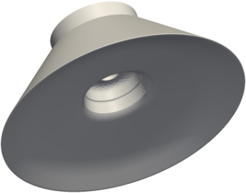 | Figure 2. Bell geometry. The bell rotates around its axis and paint is transferred from the center to the edge by the centrifugal force |
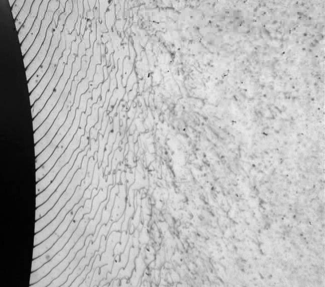 | Figure 3. Filaments of paint at the bell edge seen to the left in the picture are rotating with a tangential velocity directed downwards. The filaments stay intact for a few millimeters and then break into non-spherical droplets. Courtesy of Swerea IVF |
This paper deals with the breakup of a 2-component solvent based clear coat paint material. The viscosity of the paint has been measured to approximately 120 cP, or 0.12 Pa s with a Ford viscosity cup #4[14, Sec. 2.2.4]. The paint is a non-Newtonian liquid, but the viscosity has been verified to be approximately constant at shear rates  by measurements in a rheometer. The shear rate is expected to be at least this large during the breakup process, and the paint is therefore treated as a Newtonian liquid with the above given viscosity. The surface tension coefficient is measured to be 0.025 N/m, and the density is
  . The paint flow rate is 330 cc/min.
2.4.2. Air
The shaping air is injected through two rings of circular nozzles of diameter approximately 1 mm, located above the bell and directed downwards towards the bell edge. These nozzles are too small to resolve as it would require a huge amount of computational cells. Instead, an annulus is used as inlet condition for the air. The inlet condition is set such that the flow of momentum through the annulus is equal to that of the nozzles on the real applicator. The mass flow is larger, however, as surrounding air is entrained as the jets from the air injection nozzles slow down. The annulus has an inner radius of 35 mm and outer radius of 39 mm. The air velocity is 35 m/s directed downwards. These values correspond to a shape air of 260 slpm (standard liters per minute).
2.4.3. Simulation Setup
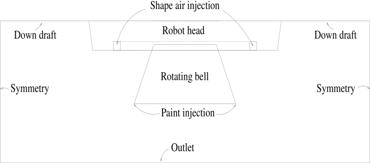 | Figure 4. Schematic description of the setup of the simulation. The simulations are performed in three spatial dimensions and a cut through the center is shown. The simulation box is shown smaller than its actual size |
The bell is modeled as a conical frustum with dimensions to match those of the bell seen in Figure 1. The base diameter is 5.5 cm, top diameter 3.375 cm and height 2.5 cm. The shape air injection is placed just behind the bell as an annulus located 0.5 cm below the top of the bell with inner diameter 7.0 cm and outer diameter 7.8 cm. The robot head is modeled as another conical frustum placed right above the air injection plane. Its lower diameter is 10 cm and the cone angle is  . Downdraft present in a paint booth is modeled as air injection on the upper boundary with a speed of 0.38 m/s directed downwards. The bottom boundary is an outlet and the four sides are modeled with symmetry boundary conditions allowing no flow in the normal direction. See Figure 4 for a schematic description of the model. The bell boundary condition is set to zero rotation velocity as the boundary layer created by the bell rotation is actually very thin, and does not extend past the primary breakup region. Instead, the swirling motion is created by the paint itself and the simulation is therefore performed with two-way coupled particles during the setup phase. During this phase correct size distributions are injected given the bell rotation speed, and a steady state solution is saved for each case considered. These solutions are later loaded in the optimization loop, where only one-way coupled simulations in a stationary air field are performed due to computational cost.The mesh consists of Cartesian cubic cells in an octree structure. That means that cells can be refined by splitting them in eight new cells, doubling the resolution in each step. The base grid is built with 30x30x10 cells with side length 20 mm. It is refined five times at the surface of the bell, so that the resolution is
  = 0.625 mm. The thickness of this refinement region is 3.1 mm. The base mesh is connected by a series of refinements one, two, three and four times towards the inner finest region. The total thickness of the refined layer is approximately 10 cm. In addition, the shape air injection zone is refined three times and a hollow cylindrical region below the bell edge is refined four times. In total
  cells are created by this refinement. The mesh in the region close to the bell can be seen in Figure 5.
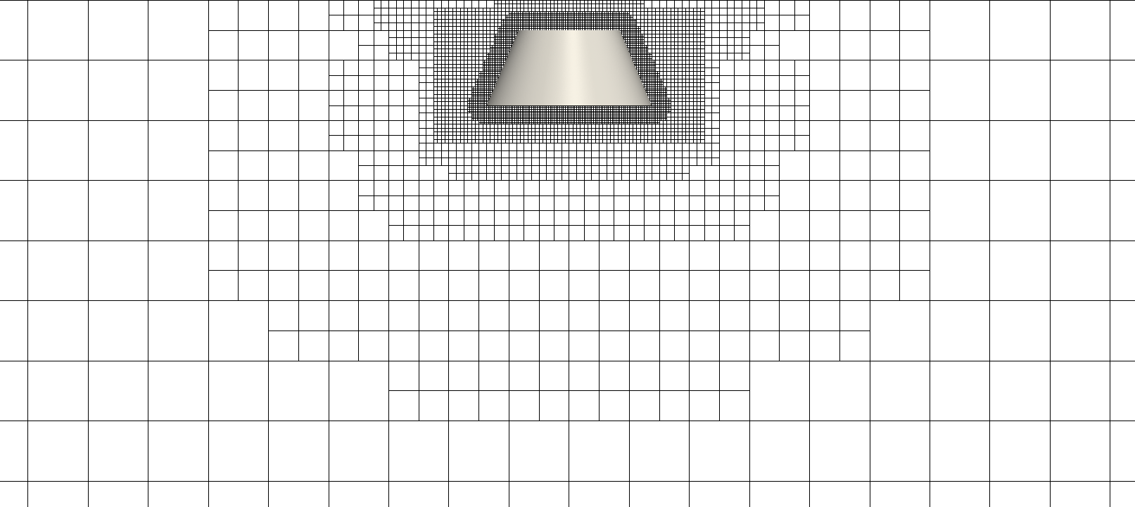 | Figure 5. Computational grid in the region close to the bell. Different levels of refinement are shown |
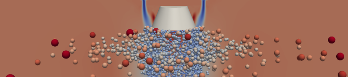 | Figure 6. Screen capture of the simulation. The color scale of the droplets is according to their radii. The droplets are not shown in their real size but substantially larger as they would otherwise be too small to display. The cut plane through the 3D domain shows the downward air velocity |
The time step used in the flow solver is adaptive such that the CFL number equals 1. For 40 kRPM bell rotation speed this amounts to  s. The particle time stepping uses an internal adaptive time step where the CFL is at most 0.5. In one time step between 50 and 150 primary droplets depending on their size are injected randomly along the periphery of the bell's lower edge.At injection each simulated droplet corresponds to exactly one physical droplet, but after breakup the simulated droplets correspond to many physical droplets each. This is done via a so-called cloud factor that determines the ratio of simulated droplets to the number of physical ones. Its value is determined by matching the mass of the simulated droplet to the corresponding physical ones. A screen capture of the bell, air velocity and paint droplets are shown in Figure 6.
2.5. Measurement Technique
The measurements were performed with a Spraytec RTS 5001 from Malvern Instruments[15] at the Fraunhofer - Institut für Produktionstechnik und Automatisierung (IPA) in Stuttgart, Germany. Figure 7 shows a schematic overview of the measurement setup. The detector is placed to the left and laser emitter to the right. In between is the bell cup spraying the paint. The bell is placed at an angle for practical reasons such that the spray does not immediately clog the lenses of the measurement equipment.The measurement technique relies on Mie scattering where laser light is scattered by the droplets and the scattering angle differs depending on the droplet radius. An array of detectors detecting particles of different size are used to create a histogram of the sizes of droplets present in the spray. The spray is directed towards the measurement zone in such a way that all droplet sizes present in the spray pass by the detector and the obtained probability density functions are valid for the whole spray.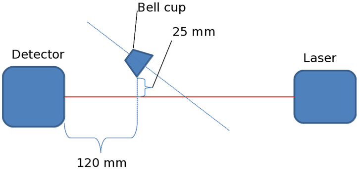 | Figure 7. Schematic description of the measurement setup |
3. Parameter Estimation
The question of finding appropriate values for the coefficients of the models such that the simulated distributions match the measurements is treated as an optimization problem, | (15) |
Here  is the vector of coefficients to the model,
  is the objective function,
  is the simulated size distribution, and
  the measured one. The argument
  to the distributions is the droplet radius as before. As objective function the discrete normalized
  error was used,
 | (16) |
where the sample points  range over the support of the measured distribution and are logarithmically spaced to capture the appearance of the distributions. N = 8192 was used in this work.The simulated droplet size distribution,
  , is evaluated by running a simulation, and then extracted by so-called Kernel Density Estimate (KDE) as described by Botev et al.[16]. Their implementation[17] of the algorithm was slightly modified to work with logarithmically spaced data and to use a specified bandwidth. The confidence interval for the distribution decreases as
  where
where  is the number of broken droplets in the simulation. This allows a trade-off between accuracy and speed, where the simulation time in the optimization was chosen such that the difference between each set of evaluated parameters was statistically significant.When the optimization of the parameters was initiated all five parameters,
  ,
, ,
,  ,
,  , and
, and  were included as free variables. It became evident by studying response surfaces obtained by Radial Basis Functions (RBF) interpolation[18, 19], however, that the value of the damping coefficient
  had negligible impact on the obtained size distributions. As described in connection to Equation (2) the
  parameter determines how strongly the modeled harmonic oscillator is damped. It therefore enters the solution of the differential equation as the time constant for the oscillations, but does not otherwise affect the breakup. It does have a second order effect as larger values mean slower breakup which allows a longer time for the droplet to be slowed down relative to the air. The relative speed to the air at the moment of breakup affects the distribution of child droplets through the Weber number, but as mentioned earlier, this is a small effect for reasonable values of
  . For this reason the standard value
  = 10 was used and the number of variables in the optimization was reduced to four:
 | (17) |
As a starting point for the optimization,  , the default values in KIVA 3[2] were used. The four parameters were then allowed to vary in a four dimensional hypercube
  . The global optimization algorithm DIRECT[20] was used to solve the optimization problem in Equation (15). To reach convergence a few hundred simulations were typically needed. Using an Intel Core i7-2600 processor running at 3.4 GHz with four parallel threads for the particle tracking required about one day to find a parameter set close to the global optimum.
4. Results
Parameters of the TAB model in Equations (5)-(6), with, and without, the modification for large viscosity by the introduction of the so-called effective Weber number defined in Equation (9), were optimized to match the measured size distributions at bell rotations speed of 30, 40 and 50 thousand revolutions per minute (RPM) simultaneously. The optimization was performed with the three cases simultaneously with the presumption that a single set of parameters can be used over a wider range of process parameters, increasing the predictive power of the model. | Figure 8. Result for the original TAB model. Measured (markers) and simulated (lines) mass distribution as a function of droplet diameter. Simulated distributions are normalized to the maximum of the measured ones. Results for 30, 40 and 50 thousand RPM |
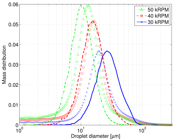 | Figure 9. Result for the modified TAB model. Measured (markers) and simulated (lines) mass distribution as a function of droplet diameter. Simulated distributions are normalized to the maximum of the measured ones. Results for 30, 40 and 50 thousand RPM |
Figure 8 shows the resulting measured and simulated distributions of mass as a function of droplet size for the original TAB model. Figure 9 shows the result for the modified model. The broken droplets were sampled when their Weber number fell below 1, at which point it was determined that further breakup would not take place. This value should be compared with the stability criterion in Equation (8) which states  as the limit below which no breakup occurs. Vibrational type of breakup may still occur at these small Weber numbers, but in the simulation with the TAB model it is extremely unlikely and this criterion does not affect the result of the simulations. Using this criterion the breakup region extends only a few centimeters from the bell as the small droplets obtained after breakup are effectively decelerated, lowering the Weber number. The total simulation time was 0.2 s and around
  primary droplets were injected during that time period. After breakup in the order of
  droplets were recorded.The optimal values of the parameters are listed in Table 1.
Table 1. Optimal Values Obtained for the Original and Modified TAB Model by the Optimization. The Default Value of the Damping Coefficient was used,
 |
| | Parameter | Original model | Modified model | KIVA 3 default |

| 7.7829 | 23.1396 | 1.2051 |

| 5.7214 | 39.5628 | 4.66671 |

| 13.0581 | 7.1598 | 0.95701 |

| 3.0745 | 5.4342 | 2.62501 |
|
|
5. Discussion
We see that the simulations agree well with the measurements. The original model seems to capture the scaling with the bell rotation speed better than the modified model, but the result for the intermediate case, 40 kRPM, for the modified model is remarkably good. As all three rotation speeds were run with the same set of parameters, the result for 30 and 50 kRPM are slightly off, however. This could most likely be avoided by tuning the parameters to the three cases individually. It is beneficial if this can be avoided, however, as the predictive power of the model is not satisfactory if each case has to be tuned individually. The dependency on the rotational speed of the bell is somewhat over-estimated by the simulations. The difference between the modes of the distributions in the measurements is slightly less than linear in rotation speed, which may be surprising. The simulations on the other hand scale slightly super-linearly. The result show that the model works with an acceptable error in the span 30-50 kRPM of rotation speed, an interval that is larger than what is usually utilized in an automotive paint shop.The tails of the distributions are less well captured than the shape in the vicinity of the modes. A little bit too few large particles are retained in the simulations, and the small dust particles with diameters  are not entirely captured. In the upper end this could be due to collisions that aggregate particles, an effect not included in the current study. This effect is believed to be small as the spray becomes progressively more dilute as droplets spread outwards. The density of particles is very low in the tails in the measurements, however, which means that the mass present there is small. This is thus an acceptable error when used as input for a simulation of the full spray painting of e.g. a car body.The primary breakup is not included in the TAB model and it therefore has to be accounted for separately. The model does not, however, appear to be particularly sensitive to the initial distribution as it seems sufficient to use a crude model for the primary breakup. This is under the assumption that the primary breakup creates droplets of which a large fraction break during the secondary breakup, which is believed to be the case.Two-way coupled simulations were run during the initialization of the optimization problem, but one-way coupled simulations were performed in the actual optimization loop. This is primarily due to the computational cost of having to update the air solution each time step due to the back coupling from the droplets to the air. The error introduced by this simplification is believed to be small as the pre-breakup relative velocity between droplets and the air is very large. The average contribution of momentum transfer is also taken into account as two-way coupled simulations are performed in the setup phase. A small widening of the simulated size distributions could however be expected by running two-way coupled simulations due to fluctuations in the relative velocities.
6. Conclusions
We have shown that the TAB model is able to capture the overall shape of the particle size distributions obtained by the rotary bell spraying technique. The tails of the distributions are less well captured, in both the upper and lower end. The distributions are slightly too narrow and as a consequence slightly over-estimate the density of particles in the middle of the distribution. In addition, the dependency on the rotational speed of the bell is somewhat over-estimated. The error is acceptably small for practical use, however, when using the simulated size distributions as input to simulation of full spray painting of realistic geometries as in[5].The modified TAB model takes into account the increased resistance to breakup introduced by the Ohnesorge number in Brodkey's relation, Equation (8). The original TAB model can therefore be assumed to give an overestimation on the breakup of viscous fluids, producing too small droplets. It is therefore important to take this effect into account when dealing with fluids of different (large) viscosities.By being able to simulate the droplet breakup the need for costly and cumbersome measurements is reduced. A limited set of measured droplet size distributions is needed for tuning the model, and it can then be used to predict changes in the size distributions without the need for new measurements. The obtained results are then used as input to full spray painting simulations that can be used by the automotive industry to reduce the time required for introduction of new car models, reduce the environmental impact and increase the quality.
ACKNOWLEDGEMENTS
This work has been conducted within the Virtual Paint Shop project. It was supported in part by the Swedish Governmental Agency for Innovation Systems, VINNOVA, through the FFI Sustainable Production Technology program, and in part by the Sustainable Production Initiative and the Production Area of Advance at Chalmers. The support is gratefully acknowledged. Henrik Söröd at Swerea IVF is acknowledged for managing the measurement campaign giving the experimental results.
References
| [1] | P. J. O'Rourke, A. A. Amsden, The TAB method for numerical calculation of spray droplet breakup, SAE paper 872089. |
| [2] | Kiva 3, http://www.lanl.gov/orgs/t/t3/codes/kiva.shtml. |
| [3] | Openfoam, http://www.openfoam.com/. |
| [4] | A. Mark, R. Rundqvist, F. Edelvik, Comparison between different immersed boundary conditions for simulation of complex fluid flows, Fluid Dynamics & Materials Processing 7 (3) (2011) 241-258. |
| [5] | A. Mark, B. Andersson, S. Tafuri, K. Engström, H. Söröd, F. Edelvik, J. S. Carlson, Simulation of electrostatic rotary bell spray painting in automotive paint shops, Atomization and Sprays, 23 (1) (2013) 25-45. |
| [6] | R. S. Brodkey, The Phenomena of Fluid Motions, Addison - Wesley Series in Chemical Engineering, Addison-Wesley Pub. Co., New York, NY, USA, 1967. |
| [7] | R. Schmehl, G. Maier, S. Wittig, CFD analysis of fuel atomization, secondary droplet breakup and spray dispersion in the premix duct of a LPP combustor, in: Eighth International Conference on Liquid Atomization and Spray Systems, Pasadena, CA, USA, 2000. |
| [8] | P. Rosin, E. Rammler, The laws governing the fineness of powdered coal, Journal of the Institute of Fuel 7 (1933) 29-36. |
| [9] | J. P. Van Doormaal, G. D. Raithby, Enhancements of the simple method for predicting incompressible fluid flows, Numerical Heat Transfer 7 (2) (1984) 147-163. |
| [10] | C. M. Rhie, W. L. Chow, Numerical study of the turbulent flow past an airfoil with trailing edge separation, AIAA Journal 21 (1983) 1525-1532. |
| [11] | L. Schiller, A. Neumann, Uber die grundlegenden berechnurgen bei der schwerkraftaufbereitung, Ver. Deutsch. Ing. 77 (1933) 318-320. |
| [12] | S. D. Cohen, A. C. Hindmarsh, CVODE, a stiff/nonstiff ODE solver in C, Computers in Physics 10 (2) (1996) 138-143. |
| [13] | A. C. Hindmarsh, P. N. Brown, K. E. Grant, S. L. Lee, R. Serban, D. E. Shumaker, C. S. Woodward, SUNDIALS: suite of nonlinear and differential/algebraic equation solvers, ACM Trans. Math. Softw. 31 (3) (2005) 363-396. |
| [14] | D. Viswanath, Viscosity of liquids: theory, estimation, experiment, and data, Springer, 2007. |
| [15] | Malvern Instruments, http://www.malvern.com. |
| [16] | Z. I. Botev, J. F. Grotowski, D. P. Kroese, Kernel density estimation via diffusion, Annals of Statistics 38 (5) (2010) 2916-2957. |
| [17] | Z. I. Botev, Kernel density estimator,http://www.mathworks.com/matlabcentral/fileexchange/14034-kernel-density-estimator. |
| [18] | H. Wendland, Scattered data approximation, Vol. 17 of Cambridge Monographs on Applied and Computational Mathematics, Cambridge University Press, Cambridge, 2005. |
| [19] | S. Jakobsson, M. Patriksson, J. Rudholm, A. Wojciechowski, A method for simulation based optimization using radial basis functions, Optimization and Engineering 11 (2010) 501-532. |
| [20] | D. R. Jones, C. D. Perttunen, B. E. Stuckman, Lipschitzian optimization without the lipschitz constant, J. Optim. Theory Appl. 79 (1993) 157-181. |
 Abstract
 Reference
 Full-Text PDF
 Full-text HTML