Yves-Simon Gloy, Robert Büllesfeld, Tobias Islam, Thomas Gries
Institut für Textiltechnik der RWTH Aachen University, Aachen, 52074, Germany
Correspondence to: Yves-Simon Gloy, Institut für Textiltechnik der RWTH Aachen University, Aachen, 52074, Germany.
| Email: |  |
Copyright © 2012 Scientific & Academic Publishing. All Rights Reserved.
Abstract
Fabric weight is an important product criterion of woven fabrics. An adequate sensor in order to monitor fabric weight during weaving is proposed in this paper. In addition, a closed control loop is designed in order to regulate fabric weight during weaving. After plant identification it is observable that the system includes a long dead time. Therefore a stable Smith predictor is designed. Stability and robustness of the Smith predictor is proven by simulation. In addition, experiments do show the necessary speed of the Smith predictor to control the fabric weight.
Keywords:
Smith-Predictor, X-Ray, Weaving, Fabric Weight
Cite this paper: Yves-Simon Gloy, Robert Büllesfeld, Tobias Islam, Thomas Gries, Application of a Smith Predictor for Control of Fabric Weight during Weaving, Journal of Mechanical Engineering and Automation, Vol. 3 No. 2, 2013, pp. 29-37. doi: 10.5923/j.jmea.20130302.02.
1. Introduction
Woven fabrics are described by rectangle crossing of so called warp and weft yarns. They are produced on looms. Modern looms uses transport mediums such as water or air to transport the weft yarn over the width of the machine. Typical weaving machine speed is around 1200 rpm, meaning also 1200 weft insertions per minute. Depending on the desired weft density (wefts per cm), typical production speed is around 0.8 m per minute. The principle of a weaving machine is shown in figure 1[1].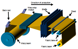 | Figure 1. Principle of a weaving machine |
Fabric weight per area is a major quality criterion for woven fabrics. It is important for example in composites for lightweight application. Setup of a loom regarding the fabric is done via the following formula  | (1) |
with Fw = mass of fabric[g/m2], F = finesse of yarn[tex], D = yarn density[threads/cm] and E = Elongation of yarns[2]. After the setup of the loom and production of the first meters of fabrics, the operator cuts samples out to the check fabric weight by lab measurements. Afterwards adaption to the weaving machines settings are carried out until the desired fabric weight is reached. So far, there is no automation known for this process. Therefore, integration of an adequate sensor to measure the fabric weight and a control system to regulate fabric weight during weaving is presented in this paper.
2. Sensor to Monitor Fabric Weight during Weaving
In order to find an adequate sensor solution to monitor fabric weight online during weaving the so called 9-Step Method was used. The 9-Step Method was developed at the Institut für Textiltechnik der RWTH Aachen University (ITA) in order to find sufficient sensor solution for textile processes[3]. As results of the use of the method, radiation absorption was determined as best solution to monitor fabric weight. A sensor using the radiation absorption is provided by the company BST ProControl GmbH, Freudenberg, Germany. The system consists of an X-ray emitter and a receiver. The X-ray emitter operates at an accelerating voltage of 5 kV and does not require permission in Germany. The sensor has a measurement range from 500 to 1000 g/m2, a resolution of 0.1 g/m2 and an accuracy of 0.3 g/m2. The principle of this radiation absorption sensor, using X-Ray, is shown in figure 2. 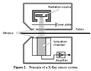 | Figure 2. Principle of a X-Ray sensor system |
Mounts were manufactured to integrate the sensor system in the weaving machine. Thus, the measuring system can be installed between fabric take-off and fabric beam. Figure 3 shows the exact measuring arrangement. 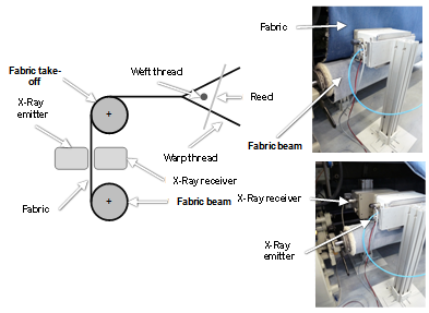 | Figure 3. Installation of the X-ray system in the weaving machine |
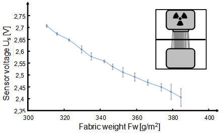 | Figure 4. Correlation between sensor signal Us and fabric weight Fw |
The sensor system was tested on an OmniPlus 800 weaving machine, manufactured by Picanol NV, Ieper, Belgium in the technical centre of the Institut für Textiltechnik der RWTH Aachen University, Aachen, Germany. The weaving machine is equipped with polyester 730dtex f2 in weft and warp yarn. The warp density is 20 threads/cm. The operating speed is 700 rpm and a twill 3/1 fabric is woven. The sensor signal is recorded while running the machine on different weft densities. Afterwards the fabric weight for each variation of the weft density is measured according to DIN EN 128181[4]. A linear correlation between fabric weight and sensor signal was found after evaluating the test results, see figure 4. Therefore the sensor system is suitable to monitor fabric weight during weaving.
3. System Identification
System analysis and thus knowledge and of the relevant system behaviour is a essential requirement to design a functional control loop. The present system is composed of the weaving machine and the X-ray sensor there to installed. Since the sensor is placed between fabric take-off and fabric beam, the system contains a dead time. Figure 5 shows the functional diagram of the controlled system. | Figure 5. Action diagram of the controlled system |
All following research was done on a weaving machine with following main parameters:• Weave pattern: twill 3/1• Weft and warp material: Polyester dtex 334/72x2• Warp density: DWarp = 20 threads/cm• Warp tension: 2.5 kNA set point A with a weaving speed of nA = 600 rpm and weft density DWeft = 16 threads/cm is defined. The operating range of the weft density is set from 12 up to 20 threads/cm.
3.1. Analysis of Weaving Machine
As shown in equation 1, fabric weight is depending on the yarn density and the elongation of the yarns. Since warp density and weft tension cannot be easily changed during weaving, the influence of warp tension and weft density was investigated in a first series of experiments.Therefore, warp tension was varied in an range of 1,75 kN up to 4 kN. During the trial speed and weft density were kept constant. Figure 6 shows the measured correlation between fabric weight and warp tension. It is visible, that there is no linear correlation between these two factors. 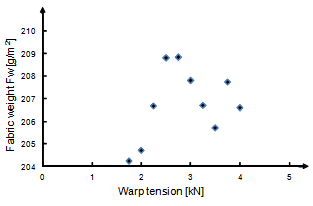 | Figure 6. Correlation between warp tension and fabric weight Fw at constant speed and weft density DWeft |
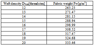
Table 1. Correlation between weft density and fabric weight
 |
| |
|
The correlation between weft density and fabric weight is gained though a series of measurements. Therefore fabric weight was determined according to DIN EN 12127 for several weft densities. Results of the measurements are shown in table 1. As shown, there is a linear linear correlation between the two parameters weft density and fabric weight.With the help of a linear curve fitting calculation, the coefficients of this linear equation  | (2) |
can be determined to KW = 8.88 g cm/m2 and Fw0 = 156.6 g/m2. It has to kept in mind, that these values will change depending on parameters like yarn material. The linear equation 2 describes the output behavior of the weaving machine. Equation 2 can be linearised under use of a taylor series in the set point A with DWeftA and FwA as  | (3) |
with the deviation values fw and d.The linearisation is independent from the set point A and therefore valid for the whole operating range due to the linear correlation of equation 2. Hence, the output behavior of the weaving machine can be described by a P element: | (4) |
3.2. Analysis of Sensor and Dead Time
Figure 7 shows the step response for a change of Fw = 334.2 g/m² (with DWeft = 20 cm-1) to Fw = 263.16 g/m² (with DWeft = 12 cm-1). The output function is smoothed using an interpolation.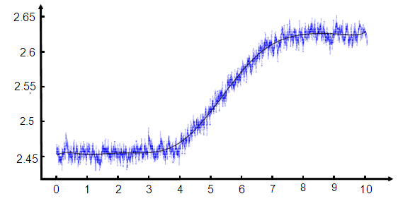 | Figure 7. Step response of X-ray sensor |
Furthermore, approximation is conducted according to Strejc[5]. With this approximation the output function is designed as PT1Tt element: | (5) |
Constants TS and dead time TtS are calculated via: | (6) |
 | (7) |
Course of step response is nearly point-symmetrically at the turning point at tW = 2.5 s. The analysis results the following values h1 = 0.0452 V, h2 = 0.1272 V and K = 0.1709 V, hence TtS = 1.3129 s and TS = 1.4197.Measurement is conducted a jump of fabric weight from von Fw = 334.2 g/m² to Fw = 263.16 g/m² and hence a difference of ΔFw = -71.04 g/m². According to the Strejc approximation Ks can be calculated as: | (8) |
Further weaving speed v is investigated: | (9) |
Figure 7 shows, that a jump in fabric weight needs around ttotal = 5.5 s until it totally passed the sensor. With the help of the speed v the length of sensor measurement range LS can be calculated as: | (10) |
Ls kept constant during all setups, since the size of sensor does not change. Constants TS und TtS can be formatted to the characteristic length LTS and LTtS as: | (11) |
 | (12) |
hence for any v TS and TtS can be calculated as: | (13) |
 | (14) |
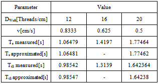
Table 2. Measured and approximated value for the sensor behaviour
 |
| |
|
Looking at the jump of fabric weight at different set points, TS and TtS are determined according to table 2.As results, the output function of sensor is described accurate with the approximation.Death time Tt depends on the length Lt between the location of fabric production and the place of the X-Ray sensor and furthermore weaving machine speed v, see figure 8.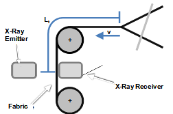 | Figure 8. Dead time length Lt in the weaving process |
Applying | (15) |
with  | (16) |
leads to the linear correlation between dead time Tt and weft density DWeft: | (17) |
Doing so, dead time distance Lt and speed n keep constant n. Length Lt was measured to 140.625 cm. As shown in equation 17 dead time depends on the parameters D and speed n. This has to be kept into account during the design of the control loop. The set point A is defined with n = 600 min-1 and DWeft = 16 cm-1. The length Lt counts 140,625 cm, hence dead time calculates to: | (18) |
The output function of the death time can be described as [Abe11]: | (19) |
3.3. Summary of System Identification
The plant can be modelled as shown in figure 9. | Figure 9. Plant model |
Therefore the output function of the control path can bed described as: | (20) |
4. Design of Control Loop
Due to the long dead time and the easy implementation a Smith predictor was chosen to design the control loop as shown in figure 10 with GC as transfer element of controller [7]. The correlation between X-Ray sensor signal and fabric weight, as analyzed in section 2, was modelled using | (21) |
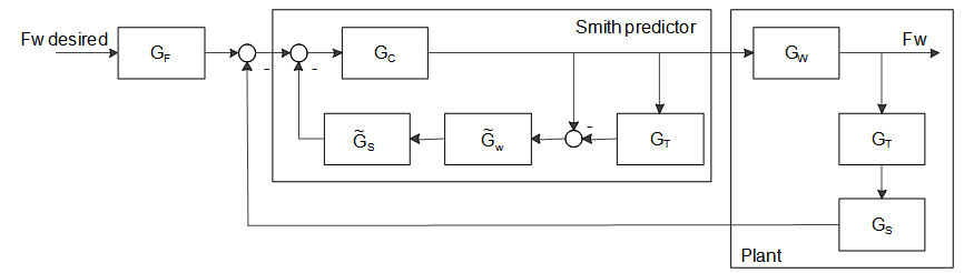 | Figure 10. Closed control loop with Smith predictor |
The output function of closed control loop is described as: | (22) |
According to[8] it is possible to design the smith predictor based on the plant without dead time. Hence, output of the smith predictor is described as: | (23) |
Within the Smith predictor, the plant is modelled as precise as possible, therefore:  | (24) |
with  as model of the plant. This is leading to the following equation of the output function of the closed control loop:
 | (25) |
The closed control loop based on the smith predictor does not show a dead time. This simplified closed control loop is shown in figure 11. 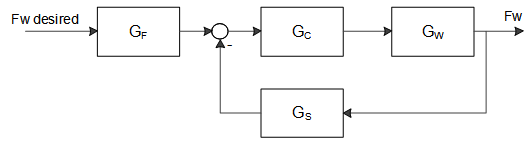 | Figure 11. Simplified closed control loop |
Due to expected instability of the Smith predictor, phase margin was set to 75°. A PI element was chosen for the controller. For the design of the controller, function PIDTUNE is used in MATLAB. The parameters of the closed control are calculated as:  and
and  Simulated output function of closed control loop with Smith predictor in comparison with a conventional PI controller is shown in figure 12. The conventional controller needs 1400 s, the Smith predictor need 20 sec to regulate the process.
  | Figure 12. Comparison step response of a simulated conventional controller and a simulated Smith predictor |
4.1. Stability of Smith Predictor
Within the set point the Smith predictor was designed for the following parameter of the transfer function according to section 3: and
and  Dead time and delay constant of the senor are independent of the used yarn material. In contrast the static amplification factors KW and KS are depending on the used yarn material They do effect the phase margin.The transfer elements GW and GS can be merged in such a way, that the control plant contains only a static amplification factor:
 The border of stability can be found in the point where the phase margin becomes zero. In order to obtain this point, the bisection method according to[9] is used.Since the closed control loop gets unstable when the static amplification factor is raised, the second starting point for the bisection method was chosen to
 In this case phase margin results in
  The closed control loop is not stable for K2. Hence, this point will be the second starting value for the bisection method. Bisection method was implemented in MATLAB with an abortion accuracy of 10-10. In this case the iteration stops after 50 cycles and delivers:
 The product of KS and KW must not be smaller than Kstabilityborder. Since
  it can be assumed that the control loop is stable.
4.2. Attenuation of Noise
In order to analyse the attenuation of noise, disturbance in the X-ray signal zs and disturbance in the fabric weight zW are intruded into the closed control loop, see figure 13. The control loop is redesigned in order to have weft density DWeft as input and fabric weight as output signal. The disturbance signal is simulated using random values within the dimension of real noise if of the sensor signal. The noise of the sensor output results in a deviation of ±6 g/m2 of the fabric weight. According to the lowest fabric weight that can be produced on the weaving machine (263 g/m2) this noise refers to relative deviation of ±2.3%. This deviation will be during the implementation of the control loop using a moving average. Noise zW affects the fabric weight in a direct way, so it cannot be damped. It is assumed to be negligible | Figure 13. Closed control loop with Smith predictor and disturbance feedforward control |
4.3. Robustness Analysis
First, robustness of the closed control loop within the static amplification factor KW is analyzed. The measurement accuracy of the static amplification factor of the weaving machine is in the dimension of 10%. This deviation will be simulated as error with in MATLAB using a second transfer function within the model of the weaving machine. Step response of Smith predictor controller with defective transfer element of the weaving machine is shown in figure 14.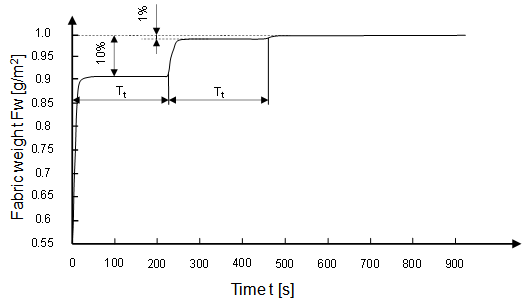 | Figure 14. Step response of Smith predictor controller with defective transfer element of the weaving machine |
The actuating variable DWeft is controlled wrong within the Smith predictor due to the inserted error. Only after the dead time passed, the control deviation is further reduced. Never less the control loop keeps stable.In the next step, similar as above, an error within the static amplification factor KS is analyzed. Step response of this redesign closed control loop is shown in figure 15.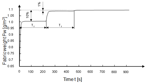 | Figure 15. Step response of Smith predictor controller with defective transfer element of the sensor |
The error within the static amplification factor of the sensor results in remaining control deviation. This deviation cannot be balanced. However the closed control loop keeps stable. In a last step, the robustness according to error within the time constants is analyzed. Also in this case, an error with maximal 10 % deviation is simulated. Step response of the closed control loop with dead time errors is shown in figure 16.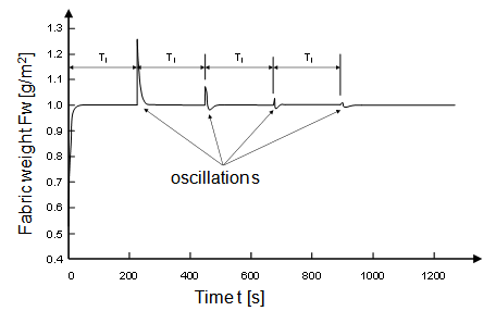 | Figure 16. Step response of Smith predictor controller with defective transfer element of the dead time |
Closed control loop keeps stable for a phase margin of 75° even if there a error within the time constants of 10 %. Never less decaying oscillations can be observed. These oscillations do have amplitude of around 25 % within the first oscillation. Period of the oscillations is equal to the dead time duration. Still, the balancing time of the Smith predictor is with 1000 s still 29 % faster than conventional closed control loop. Summarising, the Smith predictor is stable for the parameters and
and  .
.
5. Validation of Control Loop
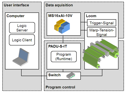 | Figure 17. System architecture for implementation of control for fabric weight into a the weaving machine |
Validation of the control loop was conducted within the Institut für Textiltechnik der RWTH Aachen University using components from company iba AG, Fürth, Germany. The X-Ray sensor is connected to ibaMS16xAI-10V, an A/D converter. In addition, the control loop was programmed using software ibaLogic-V4 and implemented on the run-time system ibaPADU-S-IT. The run-time systems use an iX86-CPU with 1600 MHz and Microsoft Windows CE as operating system with an ibaLogic-V4 Runtime engine.The communication with the weaving machine is realized using TCP/IP. Figure 17 shows the system architecture for implementation of control for fabric weight into a weaving machine.The controller is tested on an air-jet OmniPlus 800 weaving machine, manufactured by Picanol NV, Ieper, Belgium with following setup:• Weave pattern: twill 3/1• Yarn material: Polyester dtex 334/72x2• Warp density: DWarp = 20 cm-1• Warp tension: 2,5 kN First of all, the values of the plant model parameters are calculated as shown in table 3.Table 3. Calculated value of the plant
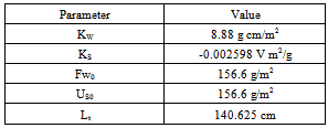 |
| |
|
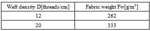
In order to calibrate the output function GF fabric weight was determined at two setting points as shown in Table 4. Calculated value of the plant
 |
| |
|
After this calibration the desired fabric weight is set to 300 g/m2 and the controller is started. The result is shown in figure 18.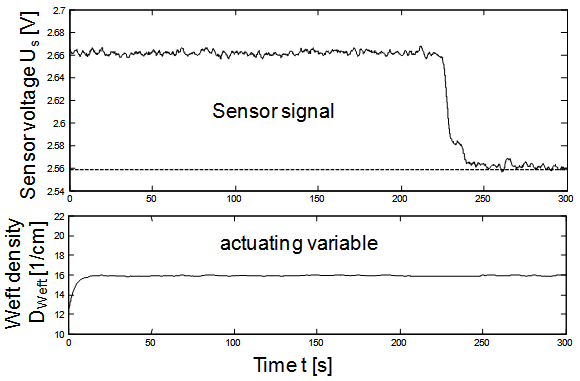 | Figure 18. Behaviour of sensor voltage and weft density during control mode |
The control loop needs around 20 s in order to regulate the fabric weight. In addition, fabric weight of the woven fabrics was determined according to DIN EN 12127 to representing a deviation of 0.93 % of the desired set value. This deviation is sufficient for industrial applications in weaving mills.
6. Conclusions
An X-Ray sensor is usable to monitor fabric weight during weaving. In addition the plant identification of the weaving machine including the sensor do show a long dead time in the system. Therefore a Smith predictor is proposed for the control of the fabric weight during weaving. The designed Smith predictor does show the necessary stability and robustness in simulations. In addition, the controller was integrated in a weaving machine and tested. The results of the experiment do show that the controller can regulate fabric weight with a necessary accuracy for industrial applications.
ACKNOWLEDGEMENTS
The authors would like to give thanks to German Research Foundation DFG for the support of the depicted research within the framework of the Cluster of Excellence “Integrative Production Technology for High-Wage Countries”. Furthermore the authors would like to give thanks to the companies• BST ProControl GmbH, Freudenberg, Germany• Picanol Nv, Ieper, Belgium• iba AG, Fürth, Germanyfor their support of this work.
References
| [1] | S. Adanur, Handbook of weaving Boca Raton, London, New York: CRC, Taylor and Francis, 2001 |
| [2] | C. Brecher, Integrative Production Technology for High-Wage Countries, Berlin, Heidelberg: Springer, 2011 |
| [3] | R. Ramakers, A. Besen, T. Gries, Konstruktionskatalog Sensortechnologie für die Online-Überwachung von Produktionsprozessen Aachen : Shaker, 2006 |
| [4] | DIN Deutsches Institut für Normung e.V., DIN EN 12127: Textile Flächengebilde - Bestimmung der flächenbezogenen Masse unter Verwendung kleiner Proben Berlin: Beuth, 1997 |
| [5] | V. Strejc, Approximation aperiodischerÜbertragungscharakteristiken, Regelungstechnik 7 (1959), pp.124-128. |
| [6] | D. Abel, Mess- und Regelungstechnik, Verlagshaus Mainz – Aachen, Aachen, 2007 |
| [7] | 0. J. Smith, A controller to overcome dead time, ISA J., vol. 6, no.2, pp. 28-33, Feb. 1959. |
| [8] | J. Lunze, Regelungstechnik 2: Mehrgrößensysteme Digitale Regelung, Heidelberg, Springer, 2008 |
| [9] | W. Dahmen, A. Reusken, Numerik für Ingenieure und Naturwissenschaftler, Berlin Heidelberg, Springer, 2007 |

 Abstract
 Reference
 Full-Text PDF
 Full-text HTML