1. Introduction

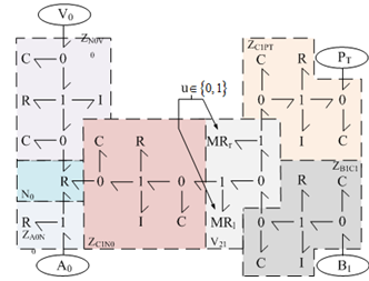
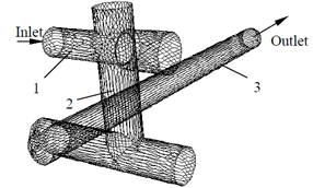
In a typical hydraulic control system, the displacement of the actuator is piloted via a control element, such as a servovalve, which is connected to the actuator by an intermediate block. Moreover, most of the other hydraulic components required by the application are also installed on this block, for example accumulators, pressure sensors, electrovalves, flow reducers, etc.. This can lead to complex intermediate blocks, which may influence the whole system dynamics. Figure 1 shows the configuration of the inner circuit of the intermediate block in our test rig. The oil from the hydraulic pump is guided into the block after a filter, and then redirected towards the servovalve. Controlled by the servovalve, the flow is supplied to the actuator through the block. Besides, the block enables the system to alternate between three different working modes via the commutation of two electrovalves (V20 and V21):

• Mode 1: a single 4-way servovalve to control the actuator;

• Mode 2: two 4-way servovalves in parallel to control the actuator;

• Mode 3: two 4-way servovalves with each servovalve used as a 3-way component to control the flow in one actuator chamber each.

According to the working mode, the oil flows in different passages and crosses several inner tubes.

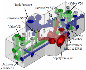
Figure 1. Configuration of the inner tubes

Most of previous studies dealing with the dynamics analysis of hydraulic servovalves and actuators[1-5] make the assumption that the effect of the intermediate block could be neglected. This assumption is reasonable for most of the conventional applications at low frequency. But for high frequency systems, this assumption becomes invalid and leads to inaccurate results. As indicated in the supplier's literature, the MOOG D765 servovalves used in the system under study have a bandwidth which can reach 500 Hz for 5%of the spool displacement with a rated flow up to 19 l/min at 70 bar pressure drop and full opening. The total inner volume of the block under consideration reaches 0.2 liter. Compared to the total actuator volume of 0.3 liter, it would influence the dynamics behavior of the hydraulic control system at high frequencies. Therefore, it makes sense to establish a dynamic model of the intermediate block in the aim to integrate it into the whole system model. This would be helpful to study the performances of the hydraulic control system at high frequencies. The main contribution of this paper is to focus on the modeling of intermediate block and to show how it may influence the hydraulic performances due to induced losses, compressibility and inertial effects. According to this study, the control performance will be finally improved, especially at high frequencies where the effect of the intermediate block volume and that of the fluid inertia in the block are involved and have a significant effect.

The modeling tool applied here to develop a dynamic model for the intermediate block is the Bond Graph modeling language[6]. This is a powerful methodology for handling complex and multidisciplinary systems with a unified graphical and mathematical form. Because of its clear architecture and flexibility to diverse problems, this method is widely adopted in various domains, i.e. mechanics[7, 8], hydraulics[9-11], thermodynamics[12, 13], robotics[14-16], etc.. With Bond Graph, the model of the intermediate block can finally be integrated into the Bond Graph model of the whole system already including a detailed model of the servovalve[17] in the range of 0 to 200 Hz working frequencies.

The model of the intermediate block should deal with the flow energy losses which are very complex. In the field of the fluid dynamics, most problems yield to nonlinear and differential representations to get an accurate result. A first way to calculate these losses is to use the Computational Fluid Dynamics (CFD) analysis. This numerical approach is based on the discretization of space and time, the continuous variables being turned to a finite set of nodal values and interpolating functions. Then, the original problem becomes an algebraic one that can be solved by computer. This method has been applied here for calculating the pressure drop in the different passages of flow in the intermediate block. However, the CFD simulation is still not usable for the simulation of the dynamics of such a system[18, 19].

This paper proposes then a method to obtain the losses parameters of the lumped-parameter model of the block based on the Bond Graph representation. It consists in considering that the inner circuits of the block are made up of associations of basic hydraulic resistance elements such as tubes, bends and bifurcations. The energy losses are then calculated using formulae and abacuses from literature for determining the pressure loss coefficients for each basic element[20, 21]. In the following, this method is called "abacus-based method" (ABM). The CFD method is then used to bring a comparison and validate the results of the proposed method.

In order to take the dynamic effect of the intermediate block into consideration, Section 2 of this paper will describe the modeling approach applied to represent accurately the intermediate block. Section 3 will introduce CFD and abacus-based methods to find the function of the energy dissipation due to the fluid flow in the block, and their results will be compared. Section 4 and 5 will study respectively the compressibility and inertial effects of the intermediate block. Some frequency response results of the simulation and experiment will be addressed in section 6 so as to demonstrate the importance of the dynamic effect of the intermediate block. Finally, section 7 will give some conclusions.

2. Modeling of the Intermediate Block

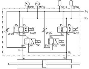
Figure 2. Scheme of the hydraulic control system setup

A scheme of the electro-hydraulic control system setup is shown in Figure 2. All components are connected on the intermediate block which guides the fluid flow according to the selected mode. The control of the electrovalves V20 and V21 allows the system to switch between the three working modes as described in the introduction.

When both electrovalves are in ON-position and the control input of one servovalve is set to 0, the control of the actuator corresponds to conventional hydraulic applications. However, in this configuration, both servovalves can be simultaneously controlled, this lead to a parallel 4-way mode which can provide a greater flow rate to the actuator. Finally, when both electrovalves are in OFF-position, the servovalves are used in 3-way mode, i.e., only one outlet port of each servovalve is connected to a chamber of the actuator. These two last modes enable the use of multivariable control strategy.

The analysis done in this paper focuses on the study of this block circuit connecting the outlet ports A and B of the servovalves and the ports V₀ and V₁ of the actuator. Five passages are then taken into consideration:

1) Passage A_i-N_i: from the port A_i of servovalve SV2i to the bifurcation N_i;

2) Passage N_i-V_i: from the bifurcation N_i to the port V_i of the chamber of the actuator;

3) Passage B_i-C_i: from the port B_i of the servovalve SV2i to port C_i of the electrovalve V2i;

4) Passage C_i-N_j: from the port C_i of the electrovalve V2i (when the valve is ON) to the bifurcation N_j;

5) Passage C_i-P_T: from the port C_i of the electrovalve V2i (when the valve is OFF) to the tank (passing through the flow reducer).

The diagram of the distribution of passages is presented in Figure 3.

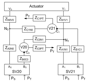
Figure 3. Diagram of the different passages of the intermediate block

While considering only the effect of the intermediate block, the influence of the losses in electrovalves and flow reducers are neglected as the flow passes through these components without bend or section change.

Each passage (noted Z in Figure 3) is modeled considering three effects: the energy dissipation (pressure drop), the compressibility, and the fluid inertia. These enable the representation of the first frequency mode for each passage.

Figure. 4 (a) shows the corresponding Bond Graph representation of a passage. The energy dissipation effect is represented by a resistor (R-element), all energy losses throughout each part of the passage being considered as a single pressure drop. These losses include the singular losses due to the local geometry (change of direction or flow area), and the frictional losses caused by the fluid viscosity. The total energy loss can be expressed as a function of the flow rate (1):

(1)

This relation will be fully developed in the next section by the means of CFD analysis and ABM.

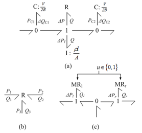
Figure 4. Bond Graph model of (a) a passage, (b) a bifurcation and (c) a valve

The fluid compressibility effect is represented by capacitors (C-elements) placed on both sides of the R-element, splitting the fluid volume of the passage into two identical volumes for model causality reason. The constitutive equation of these C-elements can be written as:

(2)

where В is the bulk modulus, and V is the whole passage volume.

The fluid inertia effect (I-element) is related to the kinetic energy of the fluid in the passage under consideration. The corresponding constitutive relationship is given by:

(3)

where l is the passage length; ρ is the fluid density; A is the equivalent section area derived from the ratio of the passage total volume and length.

A bifurcation N combines two passages together. This component can be represented by a 3-port R-element as shown in Figure 4 (b). No matter which two flow rates among the three are given, the pressure drop can be calculated according to abacus-based method according to the geometric dimensions of the bifurcation. Details will be given in the next section.

Due to the choice made for the electrovalves, the pressure losses in these components can be neglected, and they are considered to have ideal properties. As shown in Figure 4 (c), each valve is modeled by a modulated resistor (MR-element) which is controlled by a two-state command (u ∈{0, 1}). The constitutive equation of the MR-element on the left side (Figure 4 (c)) is as follows:

(4)

The equation of MR-element on the right side takes the same values but for the opposite command values in (4).

Finally, the Bond Graph model of the intermediate block is established by integrating all passages and bifurcations models. The final model is shown in Figure 5. In this model, the compressibility and inertia effects of the passage Z_A0N0 are neglected due to its small volume (nearly 2∙10^-6 m³).

Figure 5. Bond Graph model of the intermediate block for controlling a side of the actuator volume

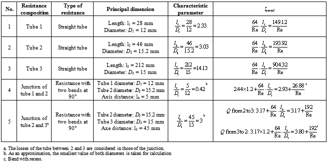
3. Energy Dissipation Calculation by Abacus-Based and CFD Methods

The relationship between the flow rate and the pressure drop is complex in hydraulic systems. The energy dissipation depends not only on the local geometry and the fluid properties, but also on the Reynolds number which is a function of the flow velocity. It does not exist a unified formula valid for all cases. The CFD analysis enables to obtain the energy dissipation in the intermediate block but this method is difficult to apply for a lumped parameter approach. Indeed, boundary conditions to be set in the numerical model are not straightforward for the inner passages as these conditions change according to what happens in all the other passages. CFD is used here only to validate the results of the abacus-based method. This is done by comparing flow rates and pressure drops characteristics for each passage and their combinations.

The CFD approach is used to determine the relationship of the flow rates and pressure drops with 3D geometric models. All passages mentioned in the previous section are exactly modeled and meshed. The boundary conditions are inlet and outlet pressure type for the single-input and single-output passages. Inlet velocity and outlet pressure boundary conditions are imposed to the bifurcations or to the passages containing a bifurcation so that the flow rate is determined at each port. Since the Reynolds number in the block is lower than 5000, laminar conditions are considered for the calculation.

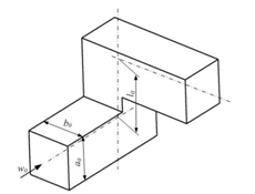
Figure 6. Element formed by two bends assembled at an angle of 90°

Table 1. Calculation of the Pressure Loss Coefficient According to ABM

Table 2. Calculation of the Pressure Drop

Figure 7. Geometric model of the passage ZC0N1

For the abacus-based approach, each passage under study is divided into basic hydraulic resistances, such as tubes, bends and bifurcations. The pressure drop of each basic element is calculated from the following equation[20]:

(5)

where ζ_total is the global pressure loss coefficient of a resistance element; w₀ is the flow velocity in the element; A₀ is the section area of the element.

The global pressure loss coefficient depends on the flow conditions by the Reynolds number, on the shape of the resistance element, and on the geometric dimensions. For the calculation of the pressure drop, it is just necessary to determine the global pressure loss coefficient by applying the empirical formulae or abacuses given in the literature[20, 21].

For example,[20] gives the following empirical formula for an element formed by two bends of same section area A₀ assembled at an angle of 90° (see in Figure 6):

(6)

where C₁ is a constant depending on the form of the tube; ζ_M is the frictional loss coefficient due to the fluid viscosity; ζ_f is the singular loss coefficient in the local resistance place. C₁ and ζ_M are obtained according to the abacuses in[20], ζ_f is given by:

(7)

where l₀ is the distance between the axes of two consecutive bends; D_H is the hydraulic diameter of the tube. Finally, the pressure drop for this element can be calculated by (5).

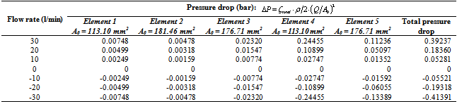
Figure 8. ABM results of pressure drops versus flow rates in the passage ZC0N1

The total pressure drop in a passage is the sum of all the pressure drops coming from the serial association of elementary hydraulic resistances. This calculation is illustrated for the passage Z_C0N1 in Figures 7, 8 and Tables 1, 2.

Figure 9 presents the distribution of total pressures and velocities in the passage Z_C0PT obtained from a commercial code (Fluent). The figure shows that the singular losses are predominant, as the flow twists violently at those places. Compared to the singular losses, the frictional ones in tubes can be nearly neglected. The magnitude of the total losses in a passage is in this case mainly associated with the singular losses.

Figure 10 presents several sets of comparative results of CFD and ABM in the main passages of the intermediate block. Both methods introduce approximately the same evolution of the pressure drop as a function of the flow rate. At low Reynolds numbers, the results of the two methods are in good agreement. However, differences between the two methods increase when the Reynolds number increases. Especially for the models made up of a small number of resistance elements, differences become non negligible, as in Figure 10 (a) and (b). These differences arise due to the following reasons:

1. The outlet flow port of the geometry is near to bends or some section change that may have effect on the flow behavior as shown in Figure 10 (a). As a result, the flow is not well developed when it passed through these places. The pressure drop obtained from CFD analysis is thus less than the one calculated from the ABM which assumes decoupled conditions.

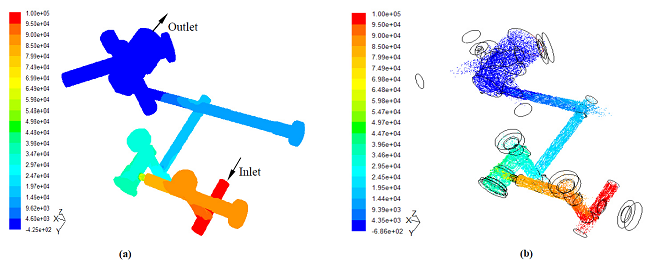
Figure 9. Total pressures profile (a) and velocity evolution (b) of the passage ZC0PT in CFD analysis

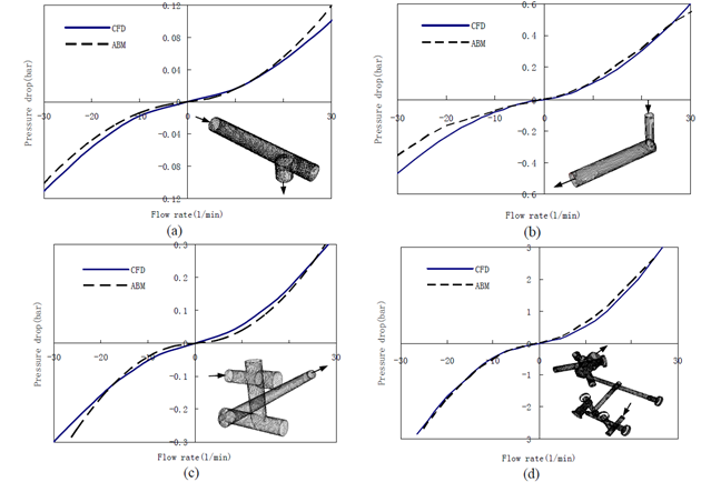
Figure 10. CFD and ABM results of pressure drops with respect to flow rates: (a) ZN0V0; (b) ZB0C0; (c) ZC0N1; (d) ZC0PT

2. The distribution of the velocity field at inlet port is not properly set. The evolution of the velocity field in the tube can cause additional energy losses.

3. The cases described in the literature do not exactly fit ours. They are used as approximation, which could lead to errors.

4. The accuracy of the CFD analysis depends on the refinement of the model, the calculation method, and the flow regime. To get a more accurate result, we could refine the mesh of the model or implement a turbulent method when the Reynolds number gets higher. But the computational time is significantly increased.

The two first effects become negligible when the energy dissipation is more important in the middle than at the two ends as in Figure 10 (d).

A set of results of the total energy dissipation in the intermediate block including all the passages between servovalves (A₁, B₀) towards the actuator chamber volume V₁ in 4-way mode is also shown in Figure 11. In this figure, the pressure drop is calculated between the port B₀ and V₁ with various flow rates at port A₁. The analytic results coming from ABM involve losses of all related passages and bifurcations. They are in good agreement with the CFD results at low flow rates imposed at port A₁ of servovalve SV21 (Figure 2). Larger differences are observed at high flow rates and can be explained by the stronger influence of the turbulent effects.

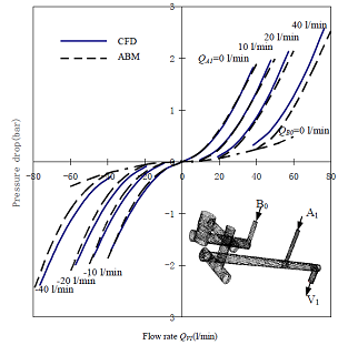
Figure 11. CFD and ABM results of pressure drop between B0 and V1 versus flow rates to or from V1 in a passage from the servovalves to the actuator chamber volume V1 (4-way mode) with various flow rates at port A1

4. Compressibility Effect of the Intermediate Block

The volume of fluid in the intermediate block between the servovalve and the actuator induces a compressibility effect. This effect will influence the dynamics of the whole system and decrease the hydraulic pulsation.

If the pressures in each passage are assumed to be identical, the volume effect of the intermediate block can be considered as an additional equivalent volume to each actuator chamber. The additional volume is the sum of the intermediate block volumes joint together. Therefore, although there is no flow in certain passages (Z_C1N0 and Z_B1C1) in mode 1, the additional volumes in modes 1 and 2 are the same as they have the same condition of the passage connection, i.e. the valves V20 and V21 in ON-position. Table 3 gives the calculated values of the additional volumes for each of the three working modes.

Table 3. Additionnal volume of each flow path Working mode Mode 1 Mode 2 Mode 3 Additional volume 0 (m3) 1.0041*10-4 1.0041*10-4 7.9754*10-5 Additional volume 1 (m3) 1.0041*10-4 1.0041*10-4 7.9754*10-5

The additional volumes 0 and 1 correspond to the flow paths from servovalve to the chamber V₀ and V₁ respectively.

Compared to the midstroke actuator volume of 1.56*10^-4m³, the volume in the intermediate block is more than half of it, and hence can not be neglected. This implies that the volume of fluid in the flow path has a significant influence on the system dynamics.

As illustrated in[22], the hydraulic natural frequency of a linear-motion hydraulic actuator can be calculated as follows:

(8)

with the hydraulic stiffness:

(9)

where В is the bulk modulus; A is the active section area of the actuator; M is the mass of the moving part; V is the actuator total volume.

Equations (8) and (9) stand for the case where the actuator is at its midstroke position. For piston at an arbitrary position, the equations should be extended to be:

(10)

where

(11)

V_Ti is the total equivalent volume of the actuator chamber i.

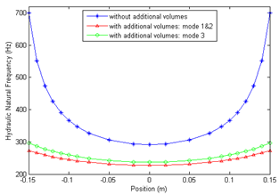
Figure 12. Evolution of the hydraulic natural frequency of the actuator according to piston position with the effect of the intermediate block volumes

Figure 12 presents the evolution of the hydraulic natural frequency of the actuator with respect to the piston position. The result shows that the additional volumes caused by the connection with the intermediate block have an important effect on the evolution of the hydraulic natural frequency. The natural frequency decreases significantly. This frequency at the end of the actuator stroke falls sharply from 700 Hz to 273 Hz for modes 1&2, and to 297 Hz for mode 3. At midstroke, the natural frequency varies from 292 Hz to 228 Hz (modes 1&2) and to 238 Hz (mode 3).

5. Inertia Effect Study of the Intermediate Block

Although the mass of fluid in the intermediate block is not important, the inertia effect can not be ignored, especially for a high performance system with a large bandwidth. This is mainly due to the small tube section in the intermediate block. The smaller the section is, the larger the velocity of the flow is, and then kinetic energy has to be taken into account.

For ease of implementation of the block inertia effect into the dynamic model and to demonstrate its importance, an equivalent mass of fluid in the block is added to the mass of the moving part of the actuator.

The kinematic energy of the hydraulic system is given by:

(12)

where ρ is the oil density; V_t1, V_t2,... are the oil volume in tube 1, 2, ...; v_t1, v_t2,... are the oil velocity in tube 1, 2, ....

The fluid velocity in the tube i can be calculated as follows:

(13)

(14)

where Q_ti is the flow rate in the tube i; Q_total is the total flow rate entering into the actuator; A_ti is the tube i section area; v is the actuator piston velocity.

Then,

(15)

The equivalent mass of the fluid in the tube i is written as:

(16)

Table 4 gives the calculated values of the total equivalent mass in each working mode. In this paper, all the calculations are under the assumption that in the mode 2 where two servovalves are used in parallel, the output flow rates of the servovalves are identical, i.e. λ equals to 0.5 in each branch passage.

Table 4. Fluid Total Equivalent Mass in Each Working Mode Working mode Mode 1 Mode 2 Mode 3 Total equivalent mass of fluid (Kg) 4.70 2.80 3.42

The moving part of the actuator has a mass M of 5.8Kg, so that the fluid equivalent mass in Table 4 is very important. This results in an obvious decrease of the hydraulic natural pulsation, similar to the effect of volume in section 4. According to (10) and (11), Figure 13 shows the evolution of the hydraulic natural frequency with consideration both of the volume and inertia effect of the intermediate block. The natural frequency values at the middle and end of stroke are presented in Table 5.

Both volume and inertia effect influence significantly the dynamics of the actuator by decreasing the hydraulic natural frequency. The results show that the volume effect has a more important impact on the natural frequency at the end of the stroke, while the inertia effect gives a proportional decrease all along the stroke.

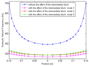
Figure 13. Evolution of the hydraulic natural frequency of the actuator with the effect of the intermediate block

6. Simulation and Experimental Results

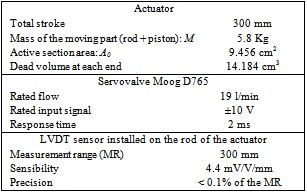
Experiments have been conducted on a test bench equipped with a high performance actuator and two large bandwidth servovalves. These hydraulic components are implanted on the intermediate block. The test rig characteristics are presented in Table 6.

Table 5. The Natural Frequency Values (Hz)

Table 6. Test Rig Characteristics

All the experimental signals are collected on an analog conditioning unit, and then digitalized at a sampling rate of 1 KHz with 16 bits precision on a dSPACE acquisition board (model DS1104).

Besides, the effect of the intermediate block is also studied by simulation (AMESim). The actuator simulation model takes into account the leakage between the two chambers with a coefficient of 1*10^-4 l/min/bar and the viscous friction with a coefficient of 400 N/(m/s). The servovalves are modeled as illustrated in[17]. The temperature of the system and the bulk modulus remain constant during the simulation.

Both experiments and simulations are implemented with a sinusoidal position input of 100 mm amplitude. The system works in mode 2, namely, two servovalves work in parallel to control the actuator. The frequency response results of the simulation and experiment are compared in Figure 14.

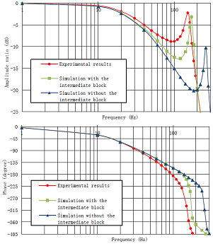
Figure 14. Frequency responses of the system from simulations and experiments in mode 2

The simulation and experimental results show a good agreement at low frequencies. However, differences between the simulation and experiment become more significant as the frequency grows until 100 Hz. Compared to the simulation results without the intermediate block, the results considering the effect of the intermediate block achieve a better coherence with the experimental ones, particularly for the resonance frequency. The above discussions demonstrate that the effect of the intermediate block takes great importance in the modeling of the hydraulic system, especially at high frequencies. The differences between the simulation and experiment can be explained by the following reasons:

a) Several parameters of the hydraulic system are difficult to obtain, e.g. the bulk modulus, friction coefficient, etc. This may induce some differences between simulation and experimental results;

b) The models used to represent some phenomena may be inefficient in some conditions, for example according to the frequency range. Indeed, dry friction and small servovalve opening can introduce behaviors that change according to the frequency (turbulence, hysteresis);

c) In the calculation of the fluid equivalent mass, the flow rate ratio λ is not strictly constant. It varies with respect to time; d) The measurement of the sensors contains noise and different types of errors, such as the LVDT phase shift.

7. Conclusions

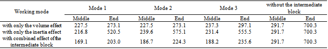
This paper investigates the modeling of an intermediate block which would probably influence the performance of the hydraulic control system at high frequencies. The model including the compressibility effects, the fluid inertia, and the energy dissipation is developed using Bond Graph approach. Besides, an approach based on abacuses to determine the energy dissipation in each passage has been used and the results have been validated by comparison with CFD analysis. The characteristics of pressure drop versus flow rate were built, and gave the necessary parameters for the lumped parameter model of the intermediate block. Moreover, the compressibility and inertia effects of the intermediate block are studied and the calculated results illustrate that they can cause an obvious decrease in the hydraulic natural frequency. According to the simulation and experiment, we demonstrate that it makes sense to consider the effect of the intermediate block while modeling a hydraulic system with high performance and large bandwidth.

References

[1]  H. E. Merritt, Hydraulic Control Systems, John Wiley & Sons, New York, 1967.
[2]  Garett A. Sohl and James E. Bobrow, “Experiments and simulations on the nonlinear control of a hydraulic servosystem,” IEEE Transactions On Contrtrol Systems Technology, vol. 7, pp. 238-247, March 1999.
[3]  P. Sekhavat, Q. Wu, and N. Sepehri, “Asymptotic Force Control of Hydraulic Actuators With Friction: Theory and Experiments,” Proc. of ASME IMECE2004, Anaheim, USA, pp. 405-412, Nov. 2004.
[4]  H. Zeng and N. Sepehri, “Tracking Control of Hydraulic Actuators Using a LuGre Friction Model Compensation,” J. Dyn. Sys. Meas. Contr., vol. 130, no. 1, pp. , Jan. 2008.
[5]  M. Choux and G. Hovland, “Adaptive Backstepping Control of Nonlinear Hydraulic-Mechanical System Including Valve Dynamics,” Modeling, Identification and Control, vol. 31, no. 1, pp. 35-44, Jan. 2010.
[6]  D. C. Karnopp and R. C. Rosenberg, System Dynamics: a Unified Approach. John Wiley & Sons, New York, 1975.
[7]  M. D. Bryant and J. Choi, “Model Based Diagnostics for Gearboxes,” Proc. of ASME/STLE IJTC2011, Los Angeles, USA, pp. 361-363, Oct. 2011.
[8]  A. K. Samantary, S. S. Dasgupta, and R. Bhattacharyya, “Bond Graph Modeling of an Internally Damped Nonideal Flexible Spinning Shaft,” J. Dyn. Sys. Meas. Contr., vol. 132, no. 6, Nov. 2010.
[9]  P. Dransfield and M. K. Teo, “Using bond graph in simulating an electro-hydraulic system,” Journal of the Franklin Institute, vol. 308, no. 3, pp. 173-184, Sep. 1979.
[10]  K. Suzuki, I. Nakamura, and J. U. Thoma, “Pressure regulator valve by Bondgraph,” Simulation Practice and Theory, vol. 7, pp. 603-611, Dec. 1999.
[11]  M. Alirand, N. Orand, and M. Lebrun, “Model Simplifications for Nonlinear Hydraulic Circuits,” Proc. of ASME IMECE2005, Orlando, USA, pp. 93-98, Nov. 2005.
[12]  F. T. Brown, “Bond-Graph Based Simulation of Thermodynamic Models,” J. Dyn. Sys. Meas. Contr., vol. 132, no. 6, Nov 2010.
[13]  F. T. Brown, “Simulating Distributed-Parameter Multiphase Thermodynamic Systems Using Bond Graphs,” Proc. of AMSE IMECE2002, New Orleans, USA, pp. 545-553, Nov. 2002.
[14]  K. Zhang, “Dynamics Design of a Planar Controllable Five Bar Mechanism Based on Genetic Algorithm,” Proc. of ASME IDETC/CIE2007, Las Vegas, USA, pp. 821-827, Sep. 2007.
[15]  M. Pellicciari, G. Berselli, and F. Leali, “Object-Oriented Modeling of Industrial Manipulators With Application to Energy Optimal Trajectory Scaling,” Proc. of IDETC/CIE2011, Washington DC, USA, pp. 997-1006, Aug. 2011.
[16]  A. K. Ghosh, A. Mukherjee and M. A. Faruqi, “Computation of Driving Efforts for Mechanisms and Robots Using Bond Graphs,” J. Dyn. Sys. Meas. Contr., vol. 113, no. 4, pp. 744-748, Dec. 1991.
[17]  Y. Xu, E. Bideaux, S. Sesmat, L. Sidhom, and X. Brun, “Hydro-mechanical model of electro-hydraulic servovalve based on Bond Graph,” Proc. of 6th FPNI-PhD Symp. West Lafayette, vol. 1, pp. 271-281, June 2010.
[18]  J. H. Ferziger, M. Peric, Computational Methods for Fluid Dynamics, Springer, 1996.
[19]  H. L. Sørensen, “Experimental and numerical analysis of flow force compensation methods for hydraulic seat valve,” The Sixth Scandinavian International Conference on Fluid Power, Tampere, Finland, May 1999.
[20]  I. E. Idelchik, Handbook of Hydraulic Resistance, CRC Begell House, 3rd Ed., 1994.
[21]  G. K. Filonenko, “An expression for the coefficient of hydraulic resistance of smooth tubes,” Izv. VTI, vol. 162, no. 10, 1948.
[22]  A. C. Morse, Electrohydraulic Servomechanisms, McGRAW-HILL, New York, USA, 1963.