1. Introduction

The Generalized Predictive Control (GPC) is one of the most favorite predictive control methods, popular in industry and also at universities. It was first published in 1987[1],[2]. The authors wanted to find one universal method to control different systems. GPC has been successfully implemented in many industrial applications, showing good performance and a certain degree of robustness. It is applicable[3] to the systems with non-minimal phase, unstable systems in open loop, systems with unknown or varying dead time, systems with unknown order and nonlinear systems approximated by linear models.

The basic idea of GPC[4],[5] is to calculate a sequence of future control signals in such a way that it minimizes a multistage cost function defined over a prediction horizon. The index to be optimized is the expectation of a quadratic function measuring the distance between the predicted system output and some reference sequence over the horizon plus a quadratic function measuring the control effort. The predictive model is carried out based on the solving Diophantine equations.

In the present paper the Adaptive Generalized Predictive Control method is designed to control a heat exchanger pilot plant and a Single Input Single Output (SISO) model is used for control purposes. The model parameters are estimated On-line using an identification algorithm based on Recursive Least Squares method. It is proved in the paper that in spite of important variations of the plant output; the developed adaptive structure maintains high level of performances (tracking, disturbance robustness and overshoot, cancellation of oscillation).

The paper is organized as follows. Section II presents the Generalized Predictive Control algorithm. Section III is devoted the description of the adaptive control algorithm. In section IV, the effectiveness and superiority of the adaptive system, is demonstrated by simulation example. Some concluding remarks end the paper.

2. Generalized Predictive Control Algorithm

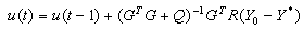
The GPC scheme[6] can be seen in Figure 1. It consists of the plant to be controlled, a reference model that specifies the desired performance of the plant, a linear model of the plant, and the Cost Function Minimization (CFM) algorithm that determines the input needed to produce the plant’s desired performance. The GPC algorithm consists of the CFM block.

The GPC system starts with the input signal, r(t), which is presented to the reference model. This model produces a tracking reference signal, w(t) that is used as an input to the CFM block. The CFM algorithm produces an output, which is used as an input to the plant. Between samples, the CFM algorithm uses this model to calculate the next control input, u(t+1), from predictions of the response from the plant’s model. Once the cost function is minimized, this input is passed to the plant. This algorithm is outlined below.

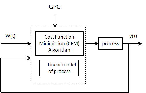Figure 1. Basic structure of GPC

When considering regulation about a particular operating point, even a non-linear plant generally admits a locally-linearized model[1] and[2]:

(1)

Where, A and B are polynomials in the backward shift operator :

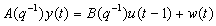
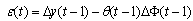
If the plant has a non-zeros dead-time the leading elements of the polynomial are zero. Where:

u(t) is the control input.

y(t) is the measured variable or output.

w(t) is a disturbance term.

In literature w(t) has been considered to be a moving average form:

Where:

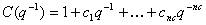In this equation is uncorrelated random sequence, and combining with (1) we obtain the CARMA (Controlled Autoregressive Moving Average):

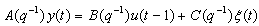(3)

Where, Δ is the differencing operator is the back shift operator such that . For simplicity in the here is chosen to be 1.

The objective of the GPC control is the output y(t) to follow some reference signal y*(t) taking into account the control effort. This can be expressed in the following cost function: locally-linearized model[1] and[2]:

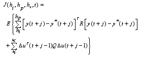(4)

Where:

h_p is the prediction horizon.

h_i is the initial horizon.

h_c is the control horizon.

y*(t) is the output reference.

R is the output weighting factor.

Q is the control weighting factor.

The control objective is to compute at each time t, control inputs that minimize the quadratic criterion for this there are two cases:

• Case 1

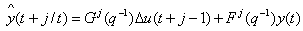
Let us first build j-step ahead predictors with following Diophantine equation:

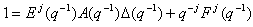(5)

Where:

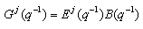
The polynomialsand are uniquely defined by: and j.

Using equation (1) and (5) we obtain:

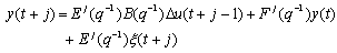(6)

The optimal predictor, given measured output data up to time t and given u(t+i) for i>1, is clearly:

(7)

Where,

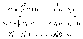
Defining 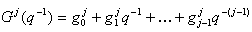then the equation above can be written in the key vector form:

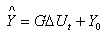(8)

Where the vectors are all :

Note that 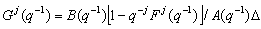so that one way to computing is simply to consider the Z-transform plant’s step-response and to take the first j terms and therefore for j=0, 1, 2 …< i independent of the particular G polynomial[1].

The matrix G is then lower-triangular of dimension :

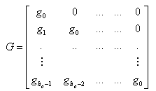Note that if the plant dead time d > 1 the first d-1 rows of the G will be null, but if instead h_i is assumed to be equal to d the leading element is non-zero[1].

From the definitions above of the vectors and with:

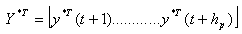The expectation of the cost-function of (4) can be written as follow:

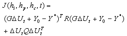(9)

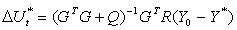
The solution, minimizing the criterion can be explicitly found, using:

(10)

it follows that:

(11)

Note that the first element of is so that the current control u(t) is given by:

(12)

• Case 2

It is possible to reduce computational burden by imposing a constant control input vector after a fixed horizon h_c

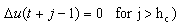In this case the vector and the matrix G become:

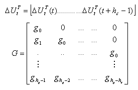
3. Adaptive Control Algorithm

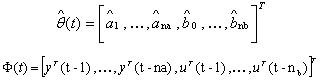
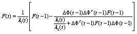
The adaptive controller which is proposed here is indirect controller. To estimate the unknown system parameters 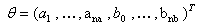the Recursive Least Squares (RLS) algorithm parameter estimates are using for tuning of the Generalized Predictive Controller. Thus, the obtained Adaptive Generalized Predictive Controller generates the current control signal.

The following (RLS) algorithm has been using:

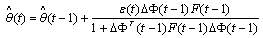(13)

(14)

(15)

Where,

Where:

is the estimation error

is the vector of data input-output

F(t) is the adaptation gain

and represents forgotten factors.

4. Simulation and Discussion

In order to illustrate the behavior of the above presented Adaptive Generalized Predictive Control, the simulation results of the heat exchanger pilot plant model obtained by using on-line identification technique[11], are given. The model is chosen as follows:

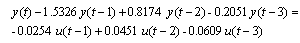(16)

Several experiments have been carried out to determine a suitable control model order an appropriate sample time for control. A tried order model (na=3, nb=2, delay=0) sampled at 1 second gave a reasonable description of a heat exchanger using on-line pilot plant dynamics.

The simulation has been done with respect to the following considerations:

• The sampling time T=1

• The plant model structure na=3, nb=2 and delay=0

• The reference is chosen as a square wave

• The polynomial chosen as

• The initial covariance matrix

4.1. Case 1: Simulation in Noise Absence Conditions

4.2. Case 2: Simulation In Noise Presence Conditions

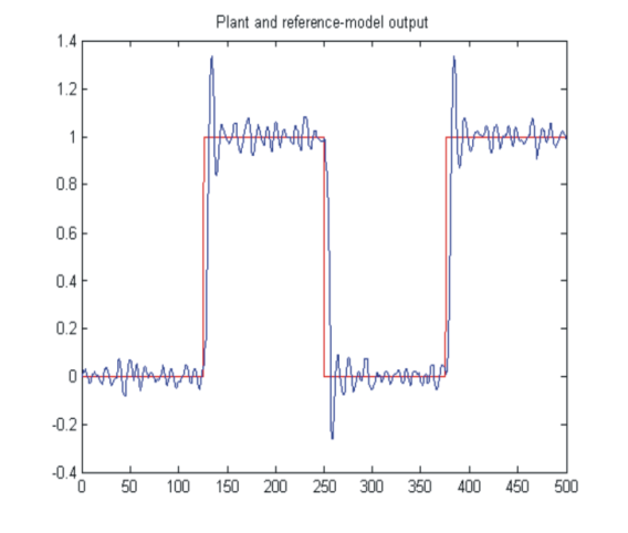
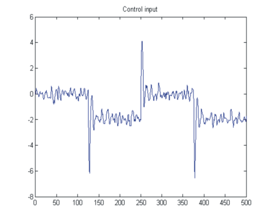
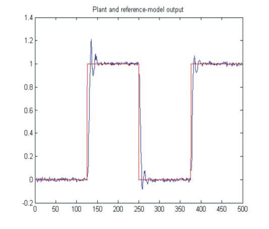
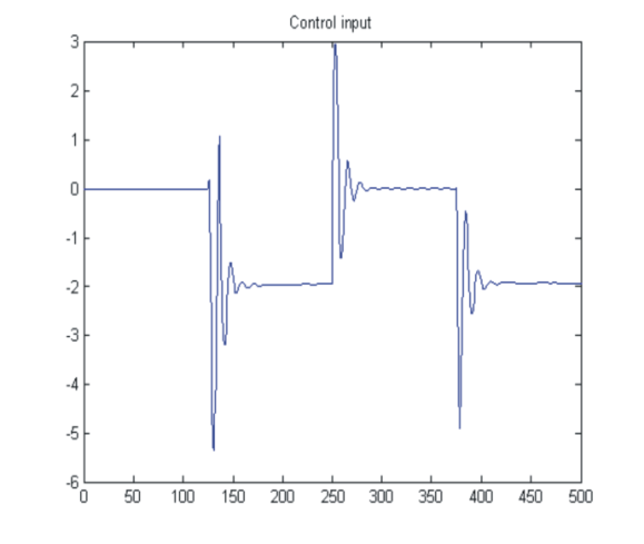
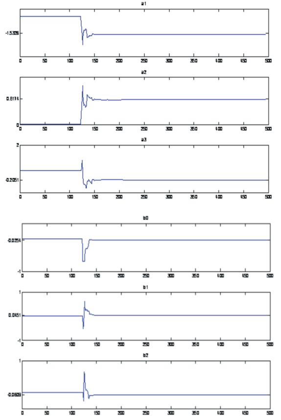
In the figures above, it can be observed the comparative results between Generalized Predictive Control and Adaptive Generalized Predictive Control, the same variation of parameters was applied.

The control performances of the Generalized Predictive Control and Adaptive Generalized Predictive Control with reference to set point changes are shown in Figures (2, 3, 4, and 5): the Adaptive Generalized Predictive Control have the same response as the Generalized Predictive Control with less oscillation.

The robustness of the control schemes to noises affecting the output has also been tested. Figures (7, 8, 9 and 10) refer to the case of white output noise (): in addition to previous considerations which are still fulfilled, it can be observed that the Adaptive Generalized Predictive Control shows better characteristics concerning the variances of the plant output and the control input.

The behavior of the model’s parameters is shown in figures 6 and 11.

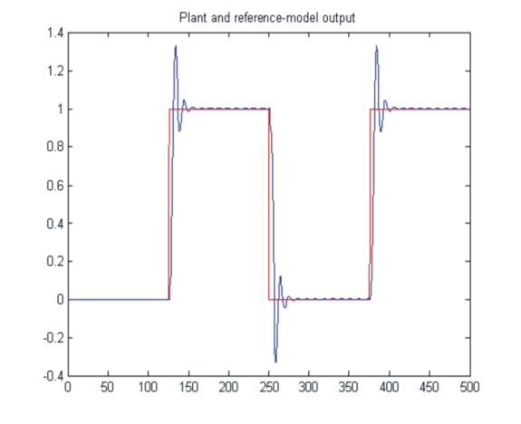Figure 2. Plant output in noise absence conditions: GPC Control

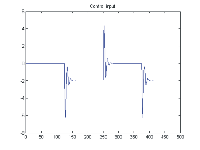Figure 3. Control input in noise absence conditions: GPC Control

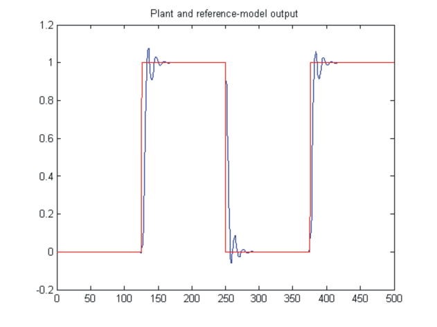Figure 4. Plant output in noise absence conditions: Adaptive predictive control

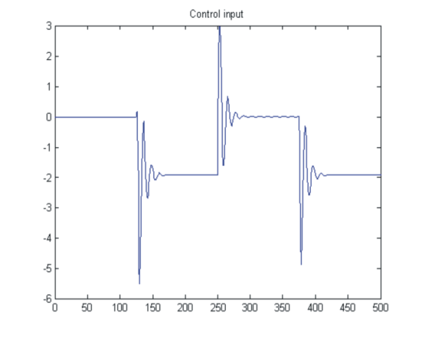Figure 5. Input control in noise absence conditions: Adaptive predictive control

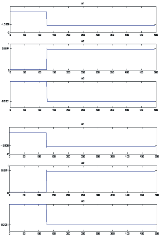Figure 6. Tuned parameters in noise absence conditions

Figure 7. Plant output in noise case: GPC Control

Figure 8. Control input in noise case: GPC Control

Figure 9. Plant output in noise case: Adaptive predictive control

Figure 10. Input control in noise case: Adaptive predictive control

Figure 11. Tuned parameters in noise case

5. Conclusions

In this paper, an Adaptive Generalized Predictive Control strategy is applied to a heat exchanger pilot plant. It has proved that, even with important variations of the plant output, the developed adaptive structure maintains a high level of performances, in terms of tracking, disturbance robustness and overshoot, cancellation of oscillation.