1. Introduction

Transportation systems pose numerous problems such as traffic accidents, traffic congestion,high energy consumption, and air pollution.One of the ways to overcome these problems is to develop automated vehicles[1-9]. Automated vehicles can contribute to the improvement of transportation through their high capacity, increased safety, low emission and high efficiency. However, unstable conditions of or faults in automated vehicles can cause serious problems; thus, it is critical for an automated vehicle to be highly reliable.

Further, an automated vehicle should be able to identify its own position with respect to surrounding obstacles. Therefore, automated vehicles are equipped with sensors for estimating their own position and detecting obstacles, and the automated mobile system controls the vehicle using the data obtained from the sensors. Some data sets are obtainedwhen the automated vehicle is under normal condition, and a few data sets are obtained when it is under unstable condition. In general it is easy to detect faults and unstable conditions using a simple algorithm. However, as the algorithm becomes complicated, it becomes difficult to detect faults in the vehicle because the number of data sets and the values to be calculated increase; further, because of the complexity of the algorithm, the obtained data tend to affect each other.

Trough investigations, S.Shladoverestablished that a system for controlling automated vehicles requireto be highly reliable because the mean time between failures (MTBF) fora human driver was very high[10]. Further, he mentioned that one of the most significant challenges faced in the research on automated vehicles was fault detection and identification. The objective of this research is to develop an algorithm for detecting faults (unstable condition) in automated vehicles and to improve the overall reliability of the vehicles.

A few researchers have concluded researches on fault detection (failure detection) algorithms and fault tolerant systems. T.H.Kerrconducteda study on fault alarm algorithm using a KalmanFilter[11]. He proposed a generalized technique for evaluating tightened upper bounds on false alarm and for correcting detection probabilities. This technique can be applied to detect any type of failure or signal. S.Schneider, et al. proposed a sensor fusion and a fault detection algorithm forlanekeeping and headway maintenanceapplications[12]. Theyused assumed fault patterns and evaluated the proposed algorithm via a simulation. In their study, fault signature was obtained virtually,and thus, the study did not involve the use of the experimentaldata. M.Hashimoto et al. proposed an algorithm for fault detection and identification of sensor-scale failure in a mobile robot, and they performed experiments by intentionally introducing faults in the robot, for evaluating the proposed algorithm[13]. Their study focused on the failure in velocity estimation, andthey evaluated the proposed algorithm usinga single-model-based Kalman Filter through experiments using a single mobile robot. With respect to fault detection at a system/device level, some algorithms for fault, failure, or unstable condition detection have already been proposed and evaluated[14-20]. In particular, statistical approaches used in these proposed algorithms have been referred to, in this study.

In this study, we first solved and updated a few patterns of data constellations under normal and unstable conditions for fault identification through real-world experiments. We performed these experiments in a public urban area, where a few pedestrians, bicycles and other robots were present. The main feature of this study is that it involves the use of experimental data obtained under real-world conditions, to develop a fault detection algorithm and evaluate its validity of it. The algorithm continuously monitors all data obtained using sensors installed in the vehicle, and if the vehicle becomes unstable the algorithm detects the unstable condition by comparing the current data with the previously stocked data using statistical approach. We have already studied the framework of the proposed algorithm using a small amount of data, and evaluated its validity[21]. This study involves the evaluation of the validity of the proposed algorithm under different conditions using a large amount of experimental data.

This paper describes an algorithm for constructing faults patterns and for detection faults, further, experiments are performed under real-world conditions, and simulation results are obtained.

2. Fault Detection Algorithm

2.1. Overview

This study focuses on the estimation of velocity and yaw angle, which are necessary tocalculate a vehicle’s position.Moreover, it does not involve obstacle detection. In this section, we explain the types of data used in the proposed algorithm, fault data obtained through the real-world experiments, the method for detection and classifying faults and unstable conditions, and the flow of the study.

2.2. Three Types of Faults

Three types of fault data sets that may lead to unstable conditions have been collected through real-world experiments; these data sets are described in section 3. It should be noted that we can obtain other types of fault data sets by performing further experiments; however, this study considers only three sets of faults data because the objective of this study is to evaluate the proposed algorithm, and these three faults can be detected manually and given that all results are known. The following are the three types of faults:

1. Communication fault

2. Encoder fault

3. Gyro fault

Communication fault (#1) indicates communication failure between a laptop and an on-board PC.

Encoder fault (#2) does not necessarily imply the failure of encoders. If a slope exists in the course taken by the vehicle, then a faulty estimate of the vehicle’s velocity is obtained because the encoders overestimate the distance covered by the vehicle while climbing a slope than while traveling on a flat road.

Gyro fault (#3) implies that the standard deviation of data obtained from a gyro is considerably higher than its specified limit. Further, the gyro requires to be calibrated before use, for determining its performance. It should be noted that the temperature was very high on the day when the data with a considerable high standard deviation has obtained from the gyro; therefore, we could not determine the main reason for the high standard deviation, but we consider that high temperature had a negative effect on the gyro.

2.3. Data for Fault Detection

The algorithm controls the automated vehicle by referring to its velocity and yaw angle, which are calculated using the different types of data obtained from the sensors. The vehicle’s position is calculated from its velocity and yaw angle.

With regard to velocitydetermination, velocity(V_e) can be estimated by measuring the difference between the current and the former values of the wheel encoder count. Velocity (V_m) can be estimated usinga map-matching algorithm[22]. The integral of deviation between the above two values is considered as the threshold value for fault detection. The integral of velocity differences (D_v) is calculated as follows:

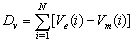(1)

The average and standard deviation were calculated by performing several experiments. Thus, the Mahalanobis distance (mD_v) of D_vcan be calculated using its average and standard deviation.

In this algorithm, if Mahalanobis distance mD_v is greater than threshold Th_D_mv, the algorithm considers that a failure in the velocity estimation flow has occurred; here, Th_D_mv is set to 2.0.

If both values are identical, it is assumed that the estimated value ofvelocity is highly reliable. On the other hand, even if both values are identical, there is a possibility that two sensors can bebroken or unstable at the same time;however, this case is not considered in this algorithm.

Further, the yaw anglecan be estimated by the differences between the values obtained from the right and left wheel encoder (R_e), a gyro sensor(R_g) and the map-matching algorithm(R_m). The integral of velocity difference is used to estimate velocity, whereas the integral of differences between the amount of change in the yaw angle during a finite period of time(200[ms]) is used to estimate the yaw angle in order to reduce the drift effort. The integrals of each yaw angle difference (E_gm ,E_egandE_em) are calculated as follows:

(2)

(3)

(4)

The average and standard deviation were also calculated by performing several experiments. Thus, the Mahalanobis distancesmE_gm, mE_eg, and mE_em of E_gm, E_eg, and E_em, respectively, can be calculatedin the same way as that used to estimate velocity. If only one of above Mahalanobis distances is greater than its threshold value (Th_mE), the algorithmconsiders that a failure in the yaw angle estimation flow has occurred.

Furthermore, velocity estimationrequires two sensors, whereas yaw angle estimationrequires three sensors. Consequently, the number of parameters increases. It is easy to detect the type of faultthat occurs by majority voting, implying that a sensor that outputs a value that is different from other sensors is unstable among all the sensors.

Hence, the number of data sets (N), is 200and the sampling frequency is 20[ms]. The distance-series data is used instead of time-series data for the fault pattern sets, because the vehicletravels continuously unless it encounters an obstacle;moreover, distance-series data does not include the data generated when the vehicles stops.

2.4. Signature of Each Fault Data Set

Through experiments, three types of fault patterns were obtained. This section describes the method for constructing a signature data set using these fault patterns.

First, we attempted to detect faults by using only the correlation coefficient in the same way as that proposed in the previous paper[12]. However, it was found that the use of only the correlation coefficient was not sufficient to correctly detect a fault because the experiments were performed under various real-world environmental conditions and multiplefaultswereexpected. Thus, along with the correlation coefficient, we also used the linearization methods to detect faults.

In order to detect faults in velocity, linear approximations of every D_v of each fault pattern were constructedusing a least square algorithm; consequently, the linear approximate equation ofD_v could be used to represent the relationship between D_v and the distance. Every D_v are shown in Fig.1.

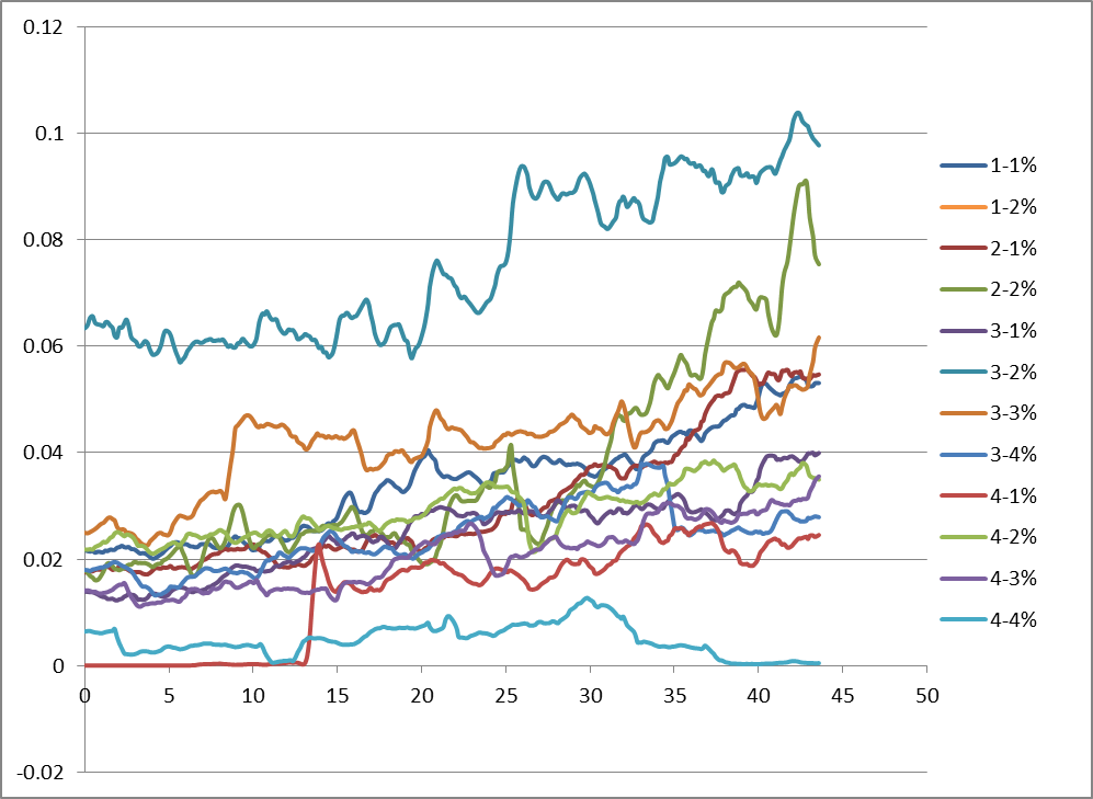Figure 1. Parameter DV obtained through experiments when the mobile robot climbs a slope

In order to detect faults in yaw angle estimation, only E_gmhasused in thealgorithm because only one type of fault occurred during several experiments. As in the case of determining faults in velocity estimation, in this case, the linear approximations of every E_gm of each fault pattern were constructed using a least square algorithm; consequently, the linear approximate equation ofE_gmcould be used to represent the relationship between E_gm and the distance.

For calculating the correlation coefficient, five parameters that represented the characteristic of each fault were selected from among all the parameters in each fault data set.

As mentioned previously, the algorithm requiresto preparean estimationof linear approximate equation and five data sets as signature data sets of each fault data set in advance in order to classify the faults.

2.5. Algorithm of Classifying Faults

In this section we first explain the algorithmfor detecting faults in velocity estimations. Figure 2 shows the flowchart of the proposed algorithm for detecting faults in velocity estimations. As described in Section 2.3, if D_mv is greater than Th_D_mv, the algorithm ascertains an unstable condition or a fault in the velocity estimation flow. Subsequently, the algorithm detects the type offaultthat occurs by comparing it with the patterns that are already stored in the algorithm. As explained in Section 2.4, the proposed algorithm uses two values that are separately calculated for detecting faults. Onevalue is obtainedusing correlation coefficient. In this algorithm, five parameters with distance-series data were used. The five values of correlation coefficient between each of the five parameterswere calculated. The expression for calculating the relative value (C_v) is given as follows:

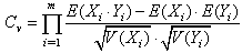(5)

The terms in this expression are defined as follows:

m: number of parameters (5 in this study)

X={Xi|i=1,2,..5}: pattern data sets stored in the algorithm (distance-series data)

Y={Yi|i=1,2,..5}: current data set (distance-series data)

V(X): standard deviation of X

E(X): average of X

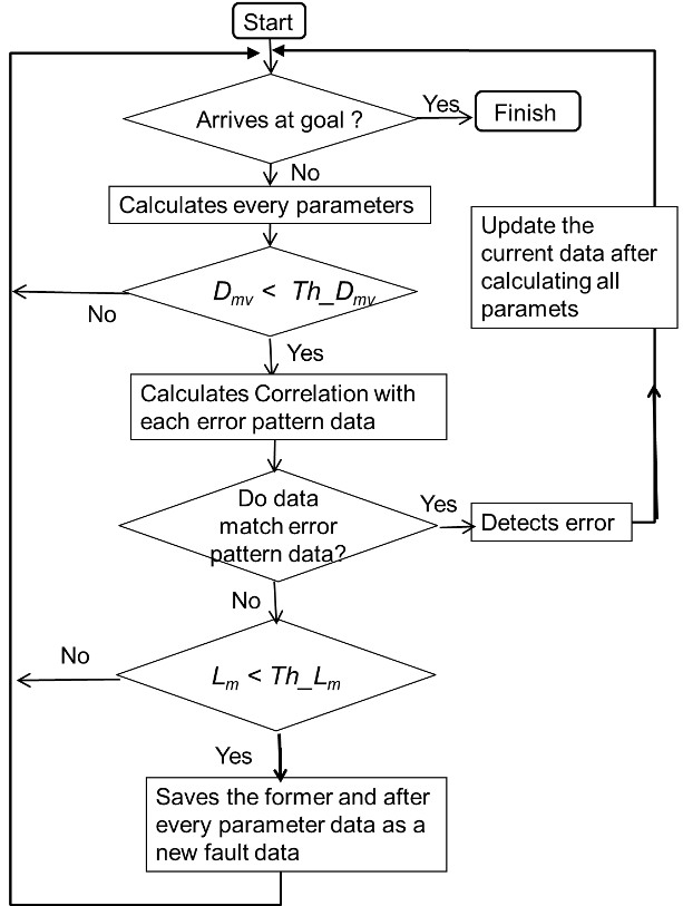Figure 2. Flow chart of proposed algorithm for detecting faults in velocity estimation

The other value used to classify faults is obtainedusing the on linearization method, and only one parameter (D_v) is used to obtain this value. The algorithmrequiresto estimate the gradient value of the linear approximate equation ofD_v using the least square algorithm before detecting faults. Further, if D_mv is greater than Th_D_mv, the algorithm estimates the liner approximate equation of D_vfromthe distance-series data; thus, the algorithm calculates the gradient and interception of the current data set. For the detection of fault in velocity estimation, only the gradient value is used. Next, the algorithm estimates the distance value (C_l) between the gradient value obtained from the linear approximate equation of the fault pattern set and the one obtained from the linear approximate equation of the current data set. If both C_v and C_l are greater than their threshold values, the algorithmascertains that afaulthas occurred. If both values are not greater than their threshold values, and the likelihood value for map-matching (L_m) is greater than its threshold (Th_L_m), then the algorithmconsiders that an unstable condition is createdowing to the missing map-matching. In other cases, the algorithmdeterminesthe occurrence of another failure and saves the current data set as a new fault pattern.

For the detection of faults in yaw angle estimation, an algorithm almost similar to that used for detecting faults in velocity estimation is used, except that this method does not involve the use of the gradient value of the linear approximate equation.

From several experimental results obtained using a gyro fault pattern, the standard deviation is found to be large and the amplitude of the deviation is larger than usual. In addition, the correlation coefficient between the gyro fault data set and the linear approximate equation calculated using its data set is very small, and it becomes difficult to estimate the liner approximate equation. Therefore, it is assumed that the correlationcoefficient may be small for the gyro fault pattern, as well.Thus, if E_gm is greater than Th_mE_gm, the algorithm estimates the linear approximate equation ofE_gmusing the current data set and calculates the correlationcoefficient (C_c) between this equation and the current data set. As in the case of fault detection in velocity estimation, five values of the correlation coefficientfor each of the five parameters are calculated and the relative value (C_v) is also calculated using equation (5). If Cc is less than the threshold value and C_y is greater than Th_C_y, the algorithmconsidersa gyro fault has occurs. In other cases, the algorithm saves the current fault pattern as a new faultdata set. In this algorithm, only one pattern is used for detecting faults in yaw angle estimation, and therefore, the method for detecting these faults is less complicated; hence, we will consider other faults or unstable conditions in our future work.

2.6. AlgorithmFlow

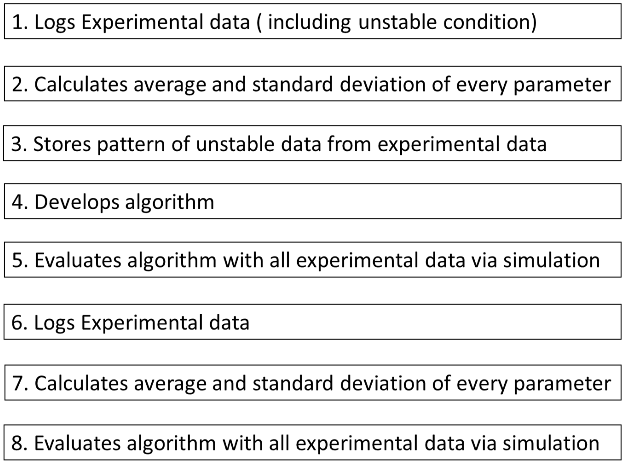Figure 3. Algorithm flow

Figure 3 shows the flow of the proposed algorithm. First, experiments were performed under real-world conditions, and all the parameters obtainedfrom experimental data, including raw data from sensors, were logged. In addition, when afault occurred during the experiments, the exact time of occurrence and the type of fault were also stored. Second, the averages and standard deviations of each value (including equations 1-4) were calculated in order to use them for determining their Mahalanobisdistance. Subsequently, as described previously, the method for detecting each type of fault was developed. Finally, the fault detection method was evaluated via a simulation using the experimental data, which includes two sets of data (logged in the first flow and newly logged). The map for map-matching was also relogged in order to evaluate the repeatability and robustness of the proposed algorithm. In the next section,we will explain the experiments and the experimental results in detail.

3.Experiments under Real-World Conditions

3.1.Instrumentation

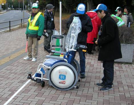
Amobile robot was usedfor the experiments. This robot was developed by modifying a wheelchair, as shown in Figure4. Figure 5 shows the system configuration of this robot. This robot can be controlled through an on-board PC using electrical signals or by a driver using a joystick. Further, it can move at a velocity of 6 [km/h]; hence, its maximum velocity was set to 4 [k/m] during the experiments, for safety reasons.

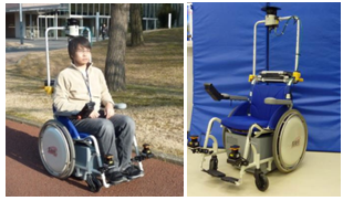Figure 4. Mobile robot

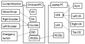Figure 5. System configuration

The mobile robot composes three laser scanner sensors (LSS), one gyro sensor, two encoder sensors for measuring the left and right wheel speeds, a laptop PC, and an on-board PC.

This robot is equippedwith a lithium-ion battery as an energy source. The battery supplies 48 [V] to all the sensors, two main motor controllers, the on-board-PC, and thelaptop PC through a DC-DC converter. This robot cantravel continuously for approximately2[h] without requiring any charging.

The robotconsists of only one laser scanner sensor mounted on top for localization. The top laser scanner sensor is horizontally mounted at a height of 1.5 [m] above the ground;the sensor is SICK LMS151[23]. The specified maximum measurement range of LMS151 is 50 [m] when the scanned objects have good reflection. From our experience,the available maximum range is 30 [m] in urban environments. The other two laser scanner sensors, which are placed under the robot, are used for obstacle detection and collision avoidance;hence, two Hokuyo UTM-30LX [24] sensors are used.The specified maximum measurement range of UTM-30LX is 30 [m] when the scanned objects have good reflection.Further, thefibre optic gyroscope sensor is placed under the seat.

The on-board PC, which is placed under the seat,is connected to the gyro sensor, two encoder sensors, an emergency switch, and a motor controller. The laptop PC is connectedto two laser scanner sensors placed under the robot through an USB and the laser scanner sensor mounted on the top of the robot through a LAN. The on-board and the laptop PCs are connected through RS-232c.

The experiments were performed in Tsukuba, Japan. The experimental course consisted of pedestrian roads. The total length of this course was approximately 1.1 [km], as shown in Figure 6-8. The surface of the course was paved with asphalt and stones. Theoperation of the robot was fully automated from the start point to the goal point. Six stop points indicated by a white line were considered, as shown in Figure 9; further, as in the case where vehicles stop at a stop sign, the robot should also stop at each white line because these stop points are intersections with poor visibility.

The mobile robot automatically stopped at each stop point, and it completely stopped operating when it reached the goal point. The experimental data that we used isthe one obtained from 100 [m] after the robot started moving to 100 [m] before it completely stopped. When the robot detects obstacles on the desired course, it automatically reduces its speed and attempts toavoid collisions with the obstacles. If the robot cannot avoid collisions, it reduces its speed and stops, and it waits until the obstacles leave the desired course.Through our experiments, we found that there are no such obstacles that the robot cannot avoid

In order to ensure safety, two researchers followed close behind the mobile robot during the experiments, and one researcher lead the robot a few meters ahead. This precaution is adopted from the previously conducted real-world experiments using a mobile robot in Tsukuba City. The total number of experiments performed while the robot travelledfrom the start point to the goal point is 17; thus, the total experimental data consists oftraveling data obtained over a course of approximately 19 [km].From among the 17 data sets, 10 sets of experimental data were used for fault detection and algorithm evaluationthe remaining seven sets were used only for algorithm evaluation.

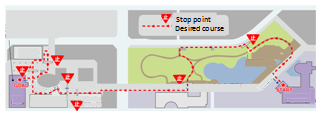Figure 6. Course map

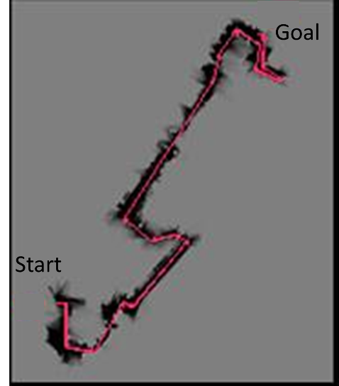Figure 7. Desired course and map for map-matching

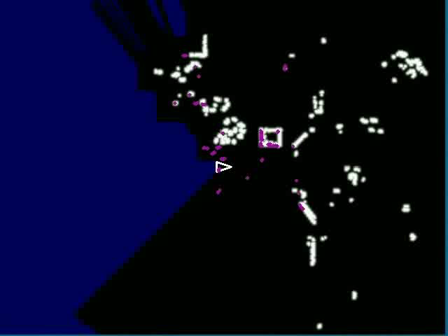Figure 8. Map-matching

Figure 9. Stop point

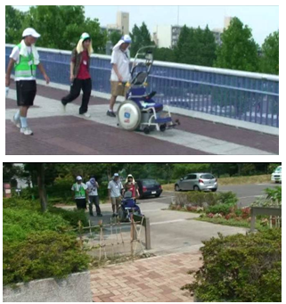Figure 10. Experimental scene

Further, the desired course of each experiment was the same; however, the other conditions such as the temperature, weather, and environment around the mobile robot were differentbecause real-world environmental conditions vary frequently.The structures used in the map-matching algorithm were almost identical; however, the number of people (walking and riding bicycle) around the robot was almost different in each experiment. Figure 10 shows an experimental scene.

4. Simulation Study Using Real-World Experimental Data

4.1. Simulationsusing Real-World Experimental Data

Simulations using real-world experimental data were performed in order to evaluate the validity of the proposed algorithm. The recognition rate of the proposed algorithm was considered to evaluate the validity of the algorithm,i.e., to obtain results indicating that the faults are detected correctly by the algorithm via simulations. Here, unknown faults are not considered because such faults were not foundwhen the algorithm was implemented.The algorithm continuously attempts to detect the type of faultthat occurs. The first detection result except for the map-matching fault is considered as the algorithm’s classifying result. The simulations wereperformed consecutively using the first to final traveling data that was obtained. The first experimental data includes three types of faults; on the other hand, the second experimental data includes only one type of fault. Nevertheless, if the proposed algorithm can detect faults using other experimental data, then the validity of the proposed algorithm can be proved.

4.2.Simulation Results and Discussion

4.2.1. First experimental data

Table 1. Simulation Result using Fault Experimental Data

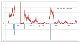Figure 11. Clipped simulation result obtained using the data of the first travel experiment (In case of fault,values -1, -2, and -3 represent missing map match, communication fault, and fault owing to slope, respectively

Table1 lists the simulation results obtained using the first experimental data. With regard to in velocity estimations, two types of faults are considered, and the algorithm correctly detects the unstable condition and classifies the faults with only one overleaping;however a smallnumber of unnecessary detections occur. It is considered that no overleaping is more important than unnecessary detections; thus, the proposed algorithm is effective in estimating faults or unstable conditions. With regard to in yaw angle estimations, only one type of fault is detected, and the algorithm correctly detects the unstable condition and classifies faults without overleaping;however, a few unnecessary detections occur here as well and therefore,further study is required in order to completely eliminate these unnecessary detection in future.

Figure 11 shows the simulation results obtained using the data of the first travel experimentfrom among 11 experiments;this result includes the communication fault and the fault during travel along a slope. The x-axis represents the distance of the robot from the start point. On y-axis, the red line represents the value of mD_v and the blue line represents the faults detected by the proposed algorithm.Values -1, -2, and -3 indicatea missing map match, a communication fault and a faultowing to the slope, respectively. In fact, the communication fault occurred at approximately 160[m], and the robot travelledalong a slope approximately 680[m] to approximately 730[m];therefore, the proposed algorithm was able to detect these faults correctly. This result thus proves the validity of the proposed algorithm.

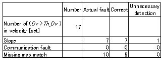
4.2.2. Second experimental data

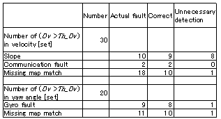
Table 2lists the simulation results obtained using the second experimental data. This simulation focuses on fault detection in velocity estimation, because faults #1 and #3 did not occur while performing the second set of experiments. This result shows that the proposed algorithm can detect the fault occurs when the robot climbs a slope with only one unnecessary detection. In addition, this algorithm detected communication faults correctly. This result proves the validity of the proposed algorithm for other experimental data, as well, thus validating its robustness. However, the algorithmrequires a few modifications in order to improve its reliability, which will be carried out in a future work.

Table 2. Simulation Results Using Second Experimental Data

5. Conclusions

This paper presents a study on fault detection for improving the reliability of automated vehicles or mobile robots. Multiple experiments were performed in a public urban area (with course distance per set beingapproximately1.1[km]), where several pedestrians, bicycles, and other robots were also present. Firstly, we solved and updated a few patterns of data constellations under normal and unstable conditions for fault detection through real-world experiments. Next, on the basis of the data obtained during the unstable condition and through other experiments the methods for deciding the threshold value ofMahalanobis distance were developed. In addition, the method of constructing the patterns of fault data and detecting faults by comparing each pattern with the relative values calculated using the correlation coefficient and linear approximate equation was proposed. Simulations wereperformed in order to evaluate the validity of the proposed algorithm, and the simulation results show that the proposed algorithm detects unstable conditions and almost correctly classifies the faults. Thus, the validity of the proposed algorithmwas proved using real-world experimental data.

In our future work,we intend to consider other fault patterns by collecting additional fault data sets through numerous experiments under real-world conditions using automated updating algorithm to construct the fault pattern sets for classifying faults.

NOMENCLATURES

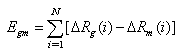
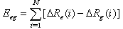
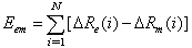
V_e: velocity estimated by measuring the difference between the current and the former values of the wheel encoder count

V_m: velocityestimated usinga map-matching algorithm

D_v :integral of velocity differencesmD_v :Mahalanobis distance of D_v

Th_D_mv,: threshold ofmD_v

R_e :yaw angle estimated by the differences between the values obtained from the right and left wheel encoder

R_g :yaw angle estimated bygyro sensor

R_m :yaw angle estimated bythe map-matching algorithm

E_gm:integrals of yaw angle difference(encoder)

E_eg:integrals of yaw angle difference (gyro sensor)

E_em :integrals of yaw angle difference (map-matching)

mE_gm :Mahalanobis distanceof E_gm

mE_eg:Mahalanobis distanceof E_eg

mE_em:Mahalanobis distanceofE_em

Th_mE: threshold ofmE_gm, mE_egandmE_em

N :number of data sets

L_m:likelihood value for map-matching

Th_L_m: threshold of the likelihood value for map-matching

C_l:distance value between the gradient value obtained from the linear approximate equation of the fault pattern set

C_c:correlationcoefficient between this equation and the current data set

C_v:expression forcalculating the relative valueX={Xi|i=1,2,..5}: pattern data sets stored in the algorithm (distance-series data)Y={Yi|i=1,2,..5}: current data set (distance-series data)V(X): standard deviation of XE(X): average of X

ACKNOWLEDGEMENTS

This study was supported by the Excellent Young Researcher Overseas Visit Program of the Japan Society of the Promotion of Science (JSPS), NSF under Cyber Physical Systems (CPS) Program (ECCS-0931669), and Energy ITS Program of NEDO.